
What Does Monetary Policy Do To Different People?
Pooyan Amir-Ahmadi, University of Illinois & Amazon
Christian Matthes, Indiana University
Mu-Chun Wang, Deutsche Bundesbank
∗
September 6, 2022
Abstract
Does monetary policy affect people differently depending on their education level, their
marital status, their race or their gender? To study this question, we use a Vector
Autoregression where monetary policy effects are identified via an instrument to study
how labor market outcomes differ across these groups after a monetary policy shock.
The response of the aggregate unemployment rate to a monetary policy shocks masks
massive heterogeneity. We find that the magnitude of the response of the difference of
unemployment rates across groups is often between 50 percent and 100 percent of the
peak response of the level of the aggregate unemployment rate.
JEL Classification: E24, E50
Key Words: Monetary Policy, Heterogeneity
∗
The views expressed in this paper are solely the responsibility of the authors and should not be interpreted
as reflecting the views of the Deutsche Bundesbank, the Eurosystem or their staff. This paper and its contents
are not related to Amazon and do not reflect the position of the company and its subsidiaries. We would
like to thank Josefine Quast and Michael Weber as well as conference participants at the Royal Economic
Society Annual Meeting for helpful comments.
1

" In fact, the distributional effects of monetary policy are complex and uncertain."
— Ben Bernanke (Bernanke (2015))
1 Introduction
One of the central questions in macroeconomics is "What does monetary policy do?"
1
More
recently, there has been an increased focus on the heterogeneous effects of monetary policy on
different socio-economic groups, and in particular how monetary policy affects labor market
outcomes across these different groups. In this paper, we focus on subgroups of the popula-
tion that are often the focus of public discourse: We study the effects of monetary policy on
subgroups of the population defined by education, gender, marital status, and race.
2
A common approach to answering this question for aggregate variables is to model the dynam-
ics of a vector of variables via a vector autoregression (VAR) and then invoke an identifying
assumption that maps forecast errors into an estimate of the monetary policy shock (see
for example the work surveyed in Christiano et al. (1999)). We use the VAR approach to
study the effects of monetary policy, but instead of focusing on aggregate variables alone,
we use U.S. micro data to augment aggregate VARs with data on labor market outcomes of
the socio-economic groups of interest. Our focus in this paper is on the unemployment rate,
where we find dramatic differences across these groups. For example, the peak effect for
men without a high school degree is double the peak effect for the aggregate unemployment
rate. Furthermore, we often find that the peak effect of the differences in the unemployment
rate across groups is at least 50 percent of the aggregate peak response. The response of the
aggregate unemployment rate to a monetary shock, thus, masks substantial heterogeneity in
the population.
Over the last decade, the economics profession has started to study the effects of monetary
policy changes on individuals. Our study focuses on time series methods and complements
work such as Bergman et al. (2022), which has an applied micro focus in terms of methods
- the authors use variation across metropolitan areas to assess the heterogeneous effects of
monetary policy on workers with different labor force attachments. Another approach uses
heterogeneous-agent versions of equilibrium models that have long been used to analyze
monetary policy (Kaplan et al., 2018; Gornemann et al., 2016; Auclert, 2019). While these
1
This is also the title of Leeper et al. (1996), which inspired our own choice of title.
2
Our choices for slicing the micro data result in overlapping groups - individuals appear in different groups
in our different exercises.
2

equilibrium models feature rich heterogeneity, this heterogeneity is usually summarized by
a few state variables at the household level (e.g. various asset positions or the current in-
come level). These models, while tremendously useful, thus do not yet contain heterogeneity
along many dimensions that (i) economists find useful to study and (ii) that are prominent
in public discourse, for example, education, gender, race, and marital status, to name just
the three dimensions we will focus on this paper.
3
Empirically, Holm et al. (2021) use Nor-
wegian micro data to empirically assess the impact of monetary policy shocks on individuals
along the wealth distribution, while Andersen et al. (2020) use Danish micro data to study
the effects of monetary policy on households along the income distribution. Both of those
papers thus focus on measures of heterogeneity commonly present in the aforementioned
equilibrium models.
The issue of heterogeneous effects of monetary policy more broadly has been touched upon
in various studies - besides the aforementioned studies, Bartscher et al. (2021) study the
effects of monetary policy on the black/white unemployment gap, while Doepke and Schnei-
der (2006) study the effects of inflation, partly controlled by monetary policy, on wealth
inequality. Coibion et al. (2017) use VARs to study the effects on inequality just like we do,
but they focus on broad summary measures of income and consumption inequality, whereas
our focus is on differences in labor market outcomes across socio-economic groups. Similar
to Coibion et al. (2017), Lenza and Slacalek (2018) analyze the effects of monetary policy
(and quantitative easing in particular) on wealth and income inequality in the Euro Area.
To identify monetary policy shocks, we exploit variation in Federal Funds futures around
Federal Open Market Committee (FOMC) meeting dates. We, hence, extend the monetary
policy instrument from Gertler and Karadi (2015). Our approach to incorporating instru-
ments in VARs is borrowed from Mertens and Ravn (2013).
The next section discusses our data. We then briefly introduce our VAR models before we
show results from our procedure for aggregate and aggregated data as a benchmark. Sec-
tion 5 contains our main results on the effects of monetary policy shocks across different
socio-economic groups.
2 Data
Our VARs combine aggregate macro data with labor market data for various socio-economic
groups that we aggregate from micro data. To aggregate the micro data, we use uniform
extracts from the Current Population Survey (CPS) outgoing rotation group provided by the
Center for Economic and Policy Research (ceprdata.org). We use micro data on hours, la-
3
One notable exception is Nakajima (2021), who studies racial inequality in such a model.
3

bor force participation, wages, and unemployment status. We extend the sample in Gertler
and Karadi (2015): the data starts in July 1979 and ends in December 2019.
4
We only
study prime age individuals throughout. Unemployment rates and labor force participation
rates are constructed as rates in the relevant groups: If, for example, everyone in one socio-
economic group who is part of the labor force had a job, the unemployment rate in that
group would be 1 irrespective of developments in other groups.
5
The macro series are the same as in Gertler and Karadi (2015): the one-year government
bond rate, the excess bond premium (Gilchrist and Zakrajsek, 2012), the log of the Consumer
Price Index (CPI) as well as the log of industrial production. All data series are seasonally
adjusted.
3 Our VAR Model
We model all vectors of variables we are studying as follows:
y
t
= m +
L
X
l=1
A
l
y
t−l
+ u
t
(1)
where we set the lag length L to 12 since we use monthly data. To identify a monetary
policy shock, we are looking to identify one column of a matrix Σ such that
u
t
= Σe
t
(2)
We borrow our approach to identification from Mertens and Ravn (2013), who show how to
use an instrument for a structural shock to identify said shock in a VAR.
6
In particular, we
use an observed measure of a monetary policy shock m
t
that has to satisfy the following two
4
Details on data sources and the construction of the instrument can be found in Appendix A.
5
We use a 3 point moving average filter to remove measurement error from the micro data. These filters
are common in signal processing, where they are called finite impulse response filters. Our benchmark is a
one-sided centered version of this filter, but we show in the appendix that our results are robust to using a
two-sided version as well.
6
As highlighted by Jentsch and Lunsford (2019), the original bootstrap procedure used by Mertens and
Ravn (2013) can be problematic. For inference, we employ the delta method proposed by Montiel Olea et al.
(2020) and subsequently used by Mertens and Ravn (2019). We show in the appendix that our results are
robust to using the parametric bootstrap of Montiel Olea et al. (2020) instead.
4

restrictions:
E(m
t
e
m
t
) = Φ [relevance condition] (3)
E(m
t
e
r
t
) = 0 [exogeneity condition] (4)
where Φ is an unknown non-zero scalar, e
m
t
is the monetary policy shock we want to identify,
e
r
t
are all other structural shocks such that [e
m
t
e
r
0
t
]
0
= e
t
, and 0 is a conformable matrix of
zeros. Our choice of instrument is the surprise in Federal Open Market Committee (FOMC)
dates in the three month ahead monthly Fed Funds futures, which is also the benchmark
choice in Gertler and Karadi (2015).
One issue to keep in mind with this approach is that the impulse responses (IRFs) are only
identified up to scale, as highlighted by Stock and Watson (2018). We scale all impulse
responses so that the initial impact of a monetary policy shock is a 25 basis point increase
in the short-term nominal interest rate. We run separate VARs for each socio-economic
group. While these VARs allow us to get a sense of different responses across different socio-
economic groups, they cannot help us to get a sense whether the differences are statistically
significant or not since we need the joint distribution of the impulse responses across socio-
economic groups for such statements. We, therefore, also run VARs where we keep the
aggregate variables as before, but now introduce the differences in labor market outcomes
between any two socio-economic groups instead of the levels of the outcomes for one group
alone. These additional VARs and their associated responses to a monetary policy shock
allow us to assess statistical significance of the differences in impulse responses by studying
the impulse responses of the differences in outcomes.
4 Aggregate Results
To assess whether our micro data is sensible, we do the following: (i) we aggregate our mi-
cro data and compare it to their aggregate counterpart, and (ii) we run a VAR with those
aggregated data as well as our standard aggregate data to check if the impulse responses to
a monetary shock look reasonable. This is especially important given the contributions by
Ramey (2016) and Bu et al. (2020), who find that identification of monetary shocks could
lead to counter-intuitive results if the sample is not informative enough about the effects of
monetary shocks.
Figure 1 shows the aggregated data versus corresponding aggregate data
7
as well as selected
results from the VAR with aggregated variables. Our aggregated unemployment rate calcu-
7
Since the responses of unemployment rates are the main focus of this paper, we focus on them here.
5
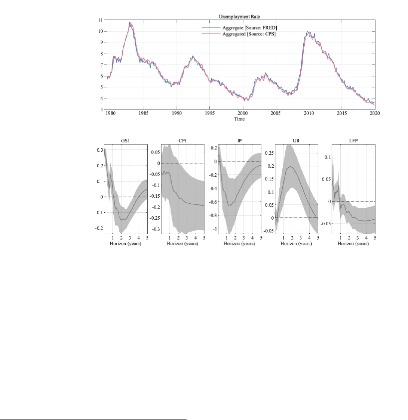
lated from CPS data tracks the aggregate unemployment rate closely. Concerning impulse
responses for aggregate and aggregated variables, our results are standard: the short-term
interest rate (labelled GS1 in Figure 1) increases on impact (this is due to our normaliza-
tion), but stays positive for one year. The price level decreases (in particular, we do not find
a price puzzle of the type that has often plagued this literature (Sims, 1992)), and industrial
production (IP) decreases. As for the aggregated variables, the unemployment rate (UR)
increases,
8
and labor force participation (LFP) shows a persistent decrease after a short in-
crease.
For the VARs with disaggregated data shown below, we display only responses of the relevant
disaggregated data. The responses of the aggregate variables in those VARs are broadly in
line with the results shown in Figure 1.
Figure 1: Impulse responses of the VAR with aggregate variables and aggregated versions of our micro
data. Error bands are 68% significance bands computed using the delta method.
5 Disaggregated Results
We now turn to describing how the labor market outcomes of various socio-economic groups
change after a monetary policy shock. The figures show the time series of the relevant labor
8
The response of the unemployment rate is similar to other results reported in the literature, see, for
example, Figure 2 in Ramey (2016).
6

market variable for the different subgroups in the top panel and the impulse responses for
each subgroup in the middle row (with the response for the aggregated variable from the
previous section also displayed in gray). The bottom row shows the impulse response of the
difference between two of the groups.
9
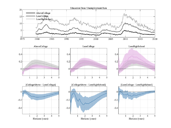
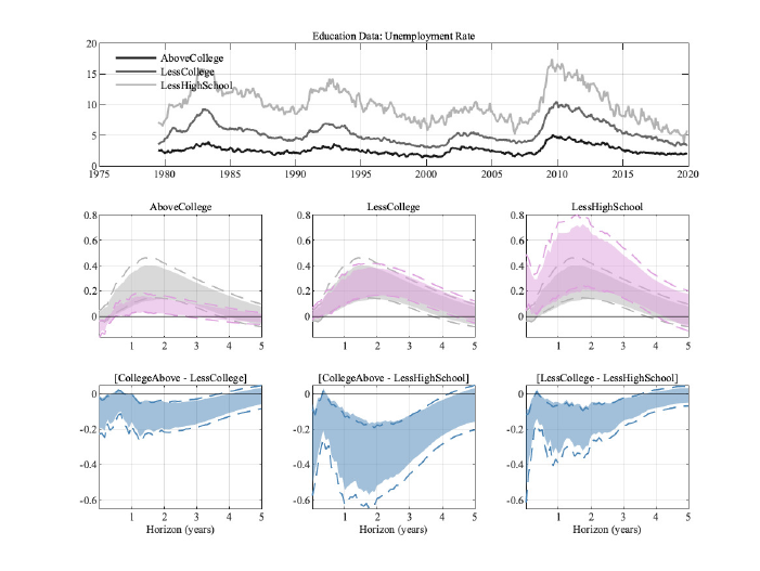
5.1 Education
Education has long been identified as a major determinant of economic outcomes. We,
therefore, begin our study of the potentially heterogeneous effects of monetary policy on
labor market outcomes by studying education. We intentionally use a relatively coarse set
of groups so that we can later interact it with other characteristics while keeping the (cross-
sectional) sample sizes meaningful - less than high school (i.e. less than 12 years of schooling),
less than a college degree (but a high school degree), and finally an undergraduate college
degree or more (titled "AboveCollege"). As is well known, the unemployment rate of people
with at least a college degree is not only substantially lower than for the other groups, but
also less volatile, as can be seen from the top panel of figure 2. The effects on the levels of
the unemployment rate differ substantially across these groups, as the unemployment rate
of those with at least a college degree reacts substantially less than for the other groups
or our aggregated unemployment rate, which we show in gray in each panel in the mid-
dle row. The response of the aggregated unemployment rate can be above or below thew
group-specific responses. We discuss this result in detail in Section 6. The bottom panel
shows that differences between the most educated group and the others are long-lived, with
the effects of monetary policy shocks being more severe the less educated a group is. The
differences between the two less educated groups, on the other hand, are neither statistically
nor economically significant. The magnitude of the response of the differences can amount
to about 0.3 percentage points of the unemployment rate, which is roughly the magnitude of
the peak response of the aggregate unemployment rate (in gray in the middle row). These
differences are economically meaningful and, as we will see below, they can become larger
as we dig deeper into the heterogeneity among different socio-economic groups.
The fact that less skilled workers are more likely to experience unemployment during reces-
sions (Heathcote et al., 2020) is thus also true for downturns driven by monetary policy.
10
9
The impulse responses in the bottom row are not just the differences of the impulse responses in the
middle row, as the VARs used to obtain the impulse responses in the bottom row use a different information
set (lags of the differences across the groups feature as endogenous variables in those VARs).
10
Further evidence for this hypothesis is provided in Jefferson (2005), who uses distributed lag models to
compute cumulative multipliers of monetary policy shocks on relative unemployment rates. He does not use
CPS data and is hence more limited in the sample length, which is just shy of 12 years in his case, whereas
we use over 30 years of data in our VAR.
7
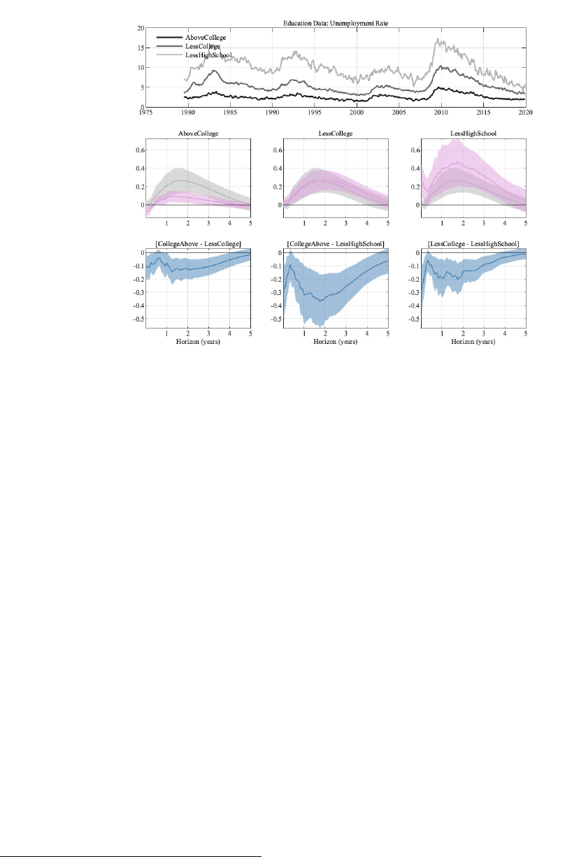
Figure 2: Results for different education levels. Error bands are 68% significance bands computed using
the delta method.
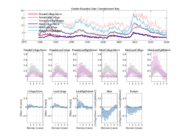
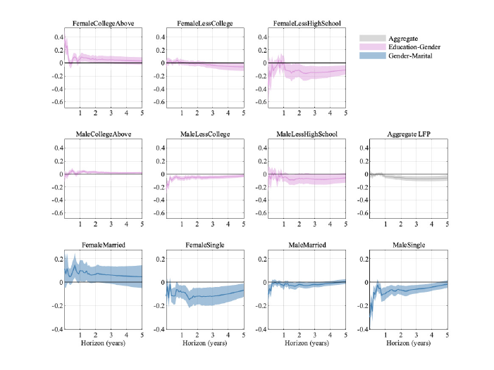
5.2 Education and Gender
We now dig deeper into the micro data to assess whether the splitting of survey participants
into education groups alone was hiding further heterogeneity. To do so, we use the same
education grouping as before, but further split by gender.
11
The results are shown in Figure
3.
While the male unemployment rate clearly increases less the higher the level of education,
for women the picture is not as clear: while the point estimate is smaller for more educated
women, the uncertainty surrounding the responses for less educated women is much larger.
Studying the IRFs of the differences in unemployment rates across these groups, we find
that when comparing the same education level across gender (the first three plots in the
third row), the unemployment rate increases significantly more for males. This increase is
larger the less educated a group is. In terms of education, the differences for a given gender
(as displayed in the last two plots of the third row) between the most educated and the
least educated groups are not only statistically significant, the maximum responses of the
differences for males are larger than the maximum response of the level of the aggregate
11
Differences in economic outcomes across genders have long been a key issue studied by economists. For
recent work, see, for example, Guvenen et al. (2020).
8
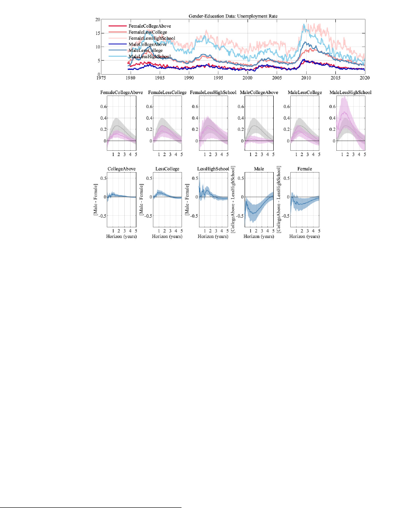
unemployment rate. For females, this response is smaller, but still close to the magnitude of
the aggregate unemployment rate response.
Figure 3: Results for different education and gender levels. Error bands are 68% significance bands
computed using the delta method.
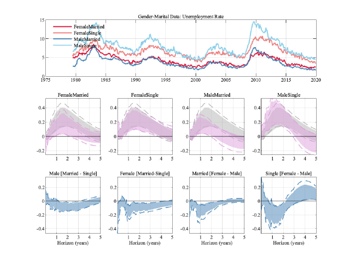
5.3 Gender and Marital Status
To understand the differential responses of males and females deeper, we now split our micro
data across both gender and marital status.
12
For both females and males, we see a larger response of singles. Singles are hit harder by a
contractionary monetary policy shock, but also benefit more from an expansionary monetary
shock. Single males are the only group in this stratification whose unemployment rate has a
larger peak response than the aggregate unemployment rate. The differences across groups
can again be as large as the peak response of the aggregate unemployment rate, as can be
seen from the bottom row of Figure 4.
12
To keep the samples sizes for the micro data reasonable, we drop the education level in this section.
9

Figure 4: Results across marital status and gender. Error bands are 68% significance bands computed
using the delta method.
5.4 Additional Results
In this section, we discuss two additional sets of results: (i) the importance of race, and (ii)
the heterogeneous effects of monetary policy shocks on labor force participation.
5.4.1 Race and Gender
Racial inequality and its interplay with monetary policy has been the focus of a number of
recent papers (Bartscher et al., 2021; Nakajima, 2021; Lee et al., 2022). While we, therefore,
chose to focus on other dimensions of heterogeneity in this paper, we want to highlight that
race is an important dimension along which there is substantial heterogeneity. Figure 5
shows the impulse responses for African-American males and females as well as the corre-
sponding Caucasian groups. The one group that has larger peak effects than the aggregate
unemployment rate is African-American males. The differences, both with respect to the ag-
gregate unemployment response, as well as to the other disaggregated groups, are startling.
Interestingly, the unemployment responses of Caucasian and African-American females are
very similar. These differences and similarities across groups mirror findings from Chetty
et al. (2019), who study the black-white income gap and find that it is driven by differences
between African-American and Caucasian males. We find that these groups also react very
10
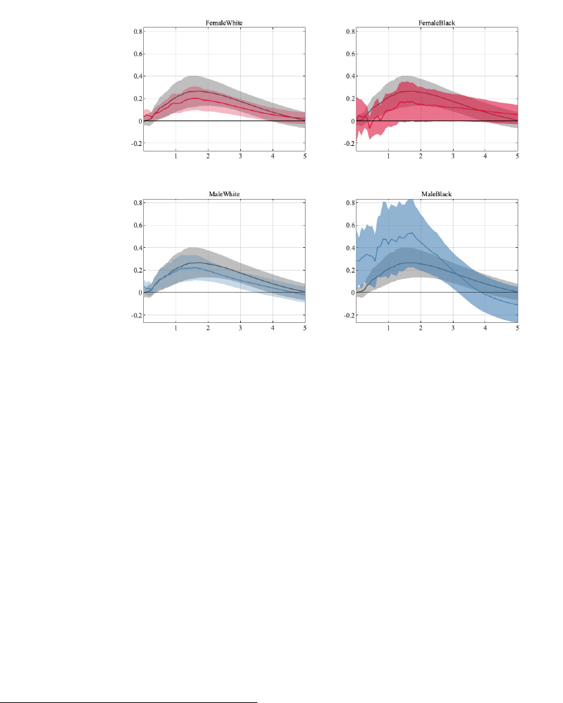
differently to monetary policy shocks. Because we use linear models, positive and negative
shocks have symmetric effects. Expansionary monetary policy shocks, thus, close the gap
in unemployment rates between African-American males and other groups according to our
results.
13
.
Figure 5: Results for gender-race UR.
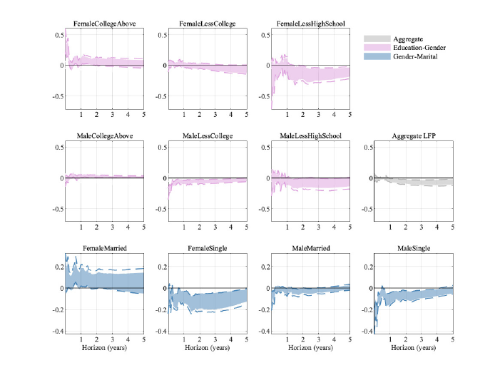
5.4.2 Labor Force Participation
While the main focus of our study is on the unemployment rate, we find it useful to also
consider how labor force participation (LFP) varies across the groups that we study, high-
lighting how our results are related to other work in macroeconomics.
We show in Figure A-10 in the Appendix the responses of the level of LFP for different
groups (as well as for our aggregated version of LFP).
14
As with the unemployment rate, various different groups have much larger swings in labor
force participation than those we see for the aggregated variable (in gray in the last panel
of the second row). However, another pattern emerges: Some groups change their labor
13
African-American unemployment rates are generally higher than for whites (see, for example, Lee et al.
(2022).
14
We moved Figure A-10 to the Appendix due to the space constraints of the journal.
11
force participation in the opposite direction relative to the aggregate response. In particular,
women with at least a college degree and those that are married increase their labor force
participation rate in response to a contractionary monetary policy shock. The same is true
for men with at least a college degree, even though their response is much more muted com-
pared to the one observed for females with the same level of education.
There is by now a growing literature highlighting how women’s labor market participation
has changed and how a woman’s labor market status may change to smooth shocks faced
by the entire family (Albanesi, 2019; Doepke and Tertilt, 2016; Gorbachev, 2016; Ellieroth,
2019). Our results show that over our sample married women entered the labor force, possi-
bly to counteract the prospect of job loss by their spouse. The aggregate negative response
of LFP seems to be mainly driven by male and female singles.
6 Disaggregation - Some Analytics
Throughout this paper we have found that group-specific impulse responses can be either
smaller or larger than the impulse response of the aggregate unemployment rate. To under-
stand possible sources of this result, consider the following stylized environment: We have
at our disposal data on a unit-variance economic shock ε
t
(for simplicity, we abstract here
from mismeasurement that we allow for in our empirical work) as well as two (mean zero)
data series x
1,t
and x
2,t
, which we can aggregate into x
t
≡ ax
1,t
+ bx
2,t
, where a and b are
non-negative weights used for aggregating micro data into one data series. To further sim-
plify this example, we (i) assume all data are independently and identically distributed (iid),
and (ii) focus on population regressions, i.e. the hypothetical scenario where we have access
to an infinite amount of data. In such a situation, we could recover the impact effect of the
monetary shock on disaggregated and aggregated variables, i.e. the population regression
coefficients α, α
1
, and α
2
in the following three regressions:
x
t
= α ε
t
+ u
t
(5)
x
1,t
= α
1
ε
t
+ u
1
t
(6)
x
2,t
= α
2
ε
t
+ u
2
t
(7)
u
t
, u
1
t
, u
2
t
are the regression residuals. The question we want to investigate is how the weights
a and b in the data construction are linked to a weight w defined via:
α = wα
1
+ (1 − w)α
2
(8)
12

This weight summarizes how heavily the impact response of x
1,t
influences the impact re-
sponse of aggregated data x
t
. Using the standard OLS formula and the fact that the variance
of ε
t
is 1, we find that
w =
a ∗ cov(x
1,t
, ε
t
) + (b − 1) ∗ cov(x
2,t
, ε
t
)
cov(x
1,t
, ε
t
) − cov(x
2,t
, ε
t
)
(9)
The weight w depends on the weights a and b used in aggregation and the larger a, the
larger the weight w. Furthermore, we can see from the data series in our earlier plots that
groups that have large IRFs usually have more volatile unemployment series. If part of that
volatility is driven by monetary shocks then the covariance of that group’s outcome with
the monetary shock is larger than for other groups, leading to an even larger weight w, as is
evident from equation (9). It is, thus, not surprising that the responses of larger groups in
the population that also have more volatile unemployment rates, such as single males, have
a large influence on the IRF of the aggregated unemployment series.
7 Conclusion
We have used standard macroeconomic identification assumptions in conjunction with well-
known micro data on labor market outcomes to shed light on how the unemployment rate
(and labor force participation) for different groups react to monetary policy shocks.
We find substantial heterogeneity across individuals in the US when it comes to the sensitivity
to monetary policy shocks. The impulse response of the differences across groups often has a
peak that is as large in magnitude as the peak of the response of the aggregate unemployment
rate. Aggregate responses, thus, mask a large amount of heterogeneity across groups: less
educated individuals show a substantially larger sensitivity to monetary policy shocks, as do
single males (with there certainly being substantial overlap between these two groups).
Dynamic equilibrium models (Auclert, 2019; Kaplan et al., 2018; Gornemann et al., 2016)
highlight channels that can lead to substantial heterogeneity in individuals’ responses to
monetary policy shocks. An interesting question for future research is whether the frictions
already present in these models are enough to account for our findings or if additional frictions
related to the groups we studied are needed. While we normalized our impulse responses
to show a contractionary monetary policy shock, this also means that these more sensitive
groups benefit more from expansionary policy than what one would expect from looking at
the aggregate impulse responses alone.
13
References
Albanesi, S. (2019, March). Changing business cycles: The role of women’s employment.
Working Paper 25655, National Bureau of Economic Research.
Andersen, A. L., N. Johannesen, M. Jørgensen, and J.-L. Peydró (2020, December). Mon-
etary Policy and Inequality. Working Papers 1227, Barcelona Graduate School of Eco-
nomics.
Auclert, A. (2019, June). Monetary Policy and the Redistribution Channel. American
Economic Review 109 (6), 2333–2367.
Bartscher, A. K., M. Kuhn, M. Schularick, and P. Wachtel (2021, January). Monetary Policy
and Racial Inequality. Staff Reports 959, Federal Reserve Bank of New York.
Bergman, N., D. A. Matsa, and M. Weber (2022, January). Inclusive Monetary Policy:
How Tight Labor Markets Facilitate Broad-Based Employment Growth. NBER Working
Papers 29651, National Bureau of Economic Research, Inc.
Bernanke, B. S. (2015, Jun). Monetary policy and inequality. Blog, Brookings Institution.
Braun, C., F. Kydland, and P. Rupert (2018, February). Quality Hours: Measuring Labor
Input. Working paper, UC Santa Barbara.
Bu, C., J. Rogers, and W. Wu (2020, February). Forward-Looking Monetary Policy and the
Transmission of Conventional Monetary Policy Shocks. Finance and Economics Discussion
Series 2020-014, Board of Governors of the Federal Reserve System (U.S.).
Chetty, R., N. Hendren, M. R. Jones, and S. R. Porter (2019, 12). Race and Economic Op-
portunity in the United States: an Intergenerational Perspective*. The Quarterly Journal
of Economics 135 (2), 711–783.
Christiano, L., M. Eichenbaum, and C. Evans (1999). Monetary policy shocks: What have
we learned and to what end? In J. B. Taylor and M. Woodford (Eds.), Handbook of
Macroeconomics, Volume 1A, pp. 65–148. Elsevier.
Coibion, O., Y. Gorodnichenko, L. Kueng, and J. Silvia (2017). Innocent Bystanders?
Monetary policy and inequality. Journal of Monetary Economics 88 (C), 70–89.
Doepke, M. and M. Schneider (2006, December). Inflation and the Redistribution of Nominal
Wealth. Journal of Political Economy 114 (6), 1069–1097.
14
Doepke, M. and M. Tertilt (2016, December). Families in Macroeconomics. In J. B. Taylor
and H. Uhlig (Eds.), Handbook of Macroeconomics, Volume 2 of Handbook of Macroeco-
nomics, Chapter 0, pp. 1789–1891. Elsevier.
Ellieroth, K. (2019). Spousal Insurance, Precautionary Labor Supply, and the Business Cycle
- A Quantitative Analysis. 2019 Meeting Papers 1134, Society for Economic Dynamics.
Gertler, M. and P. Karadi (2015, January). Monetary Policy Surprises, Credit Costs, and
Economic Activity. American Economic Journal: Macroeconomics 7 (1), 44–76.
Gilchrist, S. and E. Zakrajsek (2012, June). Credit Spreads and Business Cycle Fluctuations.
American Economic Review 102 (4), 1692–1720.
Gorbachev, O. (2016, May). Has the increased attachment of women to the labor market
changed a family’s ability to smooth income shocks? American Economic Review 106 (5),
247–51.
Gornemann, N., K. Kuester, and M. Nakajima (2016, May). Doves for the Rich, Hawks
for the Poor? Distributional Consequences of Monetary Policy. International Finance
Discussion Papers 1167, Board of Governors of the Federal Reserve System (U.S.).
Gürkaynak, R. S., K.-C. Gökçe, and S. S. Lee (2022). Stock market’s assessment of monetary
policy transmission: The cash flow effect. Journal of Finance (forthcoming).
Guvenen, F., G. Kaplan, and J. Song (2020, April). The Glass Ceiling and the Paper Floor:
Changing Gender Composition of Top Earners since the 1980s, pp. 309–373. University
of Chicago Press.
Heathcote, J., F. Perri, and G. Violante (2020, August). The Rise of US Earnings Inequality:
Does the Cycle Drive the Trend? Review of Economic Dynamics 37, 181–204.
Holm, M., P. Paul, and A. Tischbirek (2021). The Transmission of Monetary Policy under
the Microscope. Journal of Political Economy, forthcoming.
Jefferson, P. N. (2005, May). Does monetary policy affect relative educational unemployment
rates? American Economic Review 95 (2), 76–82.
Jentsch, C. and K. G. Lunsford (2019, July). The Dynamic Effects of Personal and Corporate
Income Tax Changes in the United States: Comment. American Economic Review 109 (7),
2655–2678.
15
Kaplan, G., B. Moll, and G. L. Violante (2018, March). Monetary Policy According to
HANK. American Economic Review 108 (3), 697–743.
Lee, M., C. Macaluso, and F. Schwartzman (2022). Minority Unemployment, Inflation, and
Monetary Policy. Technical report.
Leeper, E. M., C. A. Sims, and T. Zha (1996). What Does Monetary Policy Do? Brookings
Papers on Economic Activity 27 (2), 1–78.
Lenza, M. and J. Slacalek (2018, October). How does monetary policy affect income and
wealth inequality? Evidence from quantitative easing in the euro area. Working Paper
Series 2190, European Central Bank.
Mertens, K. and M. O. Ravn (2013, June). The Dynamic Effects of Personal and Corporate
Income Tax Changes in the United States. American Economic Review 103 (4), 1212–1247.
Mertens, K. and M. O. Ravn (2019, July). The Dynamic Effects of Personal and Corporate
Income Tax Changes in the United States: Reply. American Economic Review 109 (7),
2679–2691.
Montiel Olea, J. L., J. H. Stock, and M. W. Watson (2020). Inference in structural vector
autoregressions identified with an external instrument. Journal of Econometrics.
Nakajima, M. (2021). Monetary Policy with Racial Inequality. Technical report.
Ramey, V. (2016). Macroeconomic Shocks and Their Propagation. In J. B. Taylor and
H. Uhlig (Eds.), Handbook of Macroeconomics, Volume 2 of Handbook of Macroeconomics,
Chapter 0, pp. 71–162. Elsevier.
Sims, C. A. (1992, June). Interpreting the macroeconomic time series facts : The effects of
monetary policy. European Economic Review 36 (5), 975–1000.
Stock, J. H. and M. W. Watson (2018, May). Identification and Estimation of Dy-
namic Causal Effects in Macroeconomics Using External Instruments. Economic Jour-
nal 128 (610), 917–948.
16
Appendix For "What Does Monetary Policy Do To Dif-
ferent People?"
A Data
A.1 Aggregate Data Sources
We downloaded the following aggregate macroeconomic data from the FRED database with
the respective mnemonics in parentheses: Industrial Production: Total Index (INDPRO),
Consumer Price Index for All Urban Consumers (CPIAUCSL), Unemployment rate, (UN-
RATE), 1-year government bond rate (GS1), GZ excess bond premium, Average Hourly
Earnings (AHETPI), Average Weekly Hours (AWHMAN) and Labor Force Participation
Rate (CIVPART).
A.2 Micro Data Sources
We downloaded CEPR Uniform Extracts of the CPS ORG version 2.5 from CEPR data. The
sample ranges from 1979 to 2019. We drop all persons with age less than 25 or more than
54 to keep prime age workers only. All group specific labor variables are calculated based on
the final weights (fnlwgt). The hours are based on reported "usual hours" (uhourse) and we
only keep observations with positive hours.
There has been a major redesign of the CPS in 1994. This results in sudden breaks of
hours for certain demographic groups. We follow the procedure described in Braun et al.
(2018) to remove the breaks in those series. We first find the average change in each series
from December to January for all year expect 1993-1994. We then multiply the first part
of each series (January 1979 through December 1993) by a constant such that the change
from December 1993 to January 1994 is equal to the average December-January jump of
all other years. Afterwards, all series are seasonally adjusted using the default settings of
Census X-13 method implemented in Eviews 11.
A.3 Instrument Construction
The construction of the our monetary policy shock instrument is based on Gertler and
Karadi (2015) and Gürkaynak et al. (2022). In particular, we use the high frequency data
of 3 months ahead Federal Funds Future contracts provided by Gürkaynak et al. (2022) to
construct the policy instrument. We aggregate to monthly series by summing up all daily
1
surprises of the particular month. The sample of the instrument ranges from 1991M1 to
2018M12.
B Noise Filtering
To remove noise from the raw micro data we employ a 3-point moving average filter. To
highlight that our findings are robust, we show results with a one-sided filter in this appendix
(the results for the two-sided filter are in the main text). Let us denote the noisy time t raw
data by x
t
. For the two-sided filter we implement
y
t
= a
1
x
t+1
+ a
2
x
t
+ a
3
x
t−1
(A-1)
with y
t
denoting the corresponding time t noise filtered data and corresponding weights
a
1
= .25, a
2
= .5 and a
3
= .25. For the one-sided filter we implement
y
t
= a
1
x
t
+ a
2
x
t−1
+ a
3
x
t−2
(A-2)
with corresponding weights a
1
= .5, a
2
= .25 and a
3
= .25. In Figure A-1 we show the com-
parison of raw, one-sided and two-sided filtered time series of our aggregated unemployment
data.
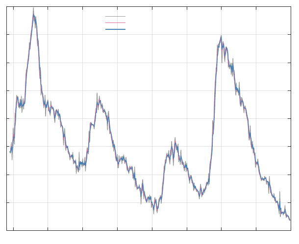
1980 1985 1990 1995 2000 2005 2010 2015 2020
Time
3
4
5
6
7
8
9
10
11
Unemployment Rate
Raw Data without Noise Filter
Two-Sided Noise Filter
One-Sided Noise Filter
Figure A-1: Raw data versus one-sided and two-sided filter applied to our aggregated unemployment data.
2
C Additional Impulse Response Graphs
C.0.1 Results with Two-sided Filter
Figure A-2: Results for different education levels. Error bands are 68% significance bands computed using
the delta method.
3
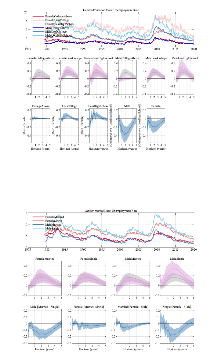
Figure A-3: Results for different education and gender levels. Error bands are 68% significance bands
computed using the delta method.
Figure A-4: Results across marital status and gender. Error bands are 68% significance bands computed
using the delta method.
4
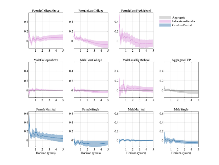
Figure A-5: Impulse responses of the labor force participation rate across groups. Error bands are 68%
significance bands computed using the delta method.
5
D Labor Force Participation
Figure A-10: Impulse responses of the labor force participation rate across groups. Error bands are 68%
significance bands computed using the delta method.
10
