
Board of Governors of the Federal Reserve System
Monetary Policy rePort
February 23, 2018
For use at 11:00 a.m., EST
February 23, 2018

Letter of transmittaL
B G
F R S
Washington, D.C., February 23, 2018
T P S
T S H R
The Board of Governors is pleased to submit its Monetary Policy Report pursuant to
section 2B of the Federal Reserve Act.
Sincerely,
Jerome H. Powell, Chairman
Adopted effective January24, 2012; as amended effective January30, 2018
The Federal Open Market Committee (FOMC) is rmly committed to fullling its statutory
mandate from the Congress of promoting maximum employment, stable prices, and moderate
long-term interest rates. The Committee seeks to explain its monetary policy decisions to the public
as clearly as possible. Such clarity facilitates well-informed decisionmaking by households and
businesses, reduces economic and nancial uncertainty, increases the eectiveness of monetary
policy, and enhances transparency and accountability, which are essential in a democratic society.
Ination, employment, and long-term interest rates uctuate over time in response to economic and
nancial disturbances. Moreover, monetary policy actions tend to inuence economic activity and
prices with a lag. Therefore, the Committee’s policy decisions reect its longer-run goals, its medium-
term outlook, and its assessments of the balance of risks, including risks to the nancial system that
could impede the attainment of the Committee’s goals.
The ination rate over the longer run is primarily determined by monetary policy, and hence the
Committee has the ability to specify a longer-run goal for ination. The Committee rearms its
judgment that ination at the rate of 2percent, as measured by the annual change in the price
index for personal consumption expenditures, is most consistent over the longer run with the
Federal Reserve’s statutory mandate. The Committee would be concerned if ination were running
persistently above or below this objective. Communicating this symmetric ination goal clearly to the
public helps keep longer-term ination expectations rmly anchored, thereby fostering price stability
and moderate long-term interest rates and enhancing the Committee’s ability to promote maximum
employment in the face of signicant economic disturbances. The maximum level of employment
is largely determined by nonmonetary factors that aect the structure and dynamics of the labor
market. These factors may change over time and may not be directly measurable. Consequently,
it would not be appropriate to specify a xed goal for employment; rather, the Committee’s policy
decisions must be informed by assessments of the maximum level of employment, recognizing that
such assessments are necessarily uncertain and subject to revision. The Committee considers a
wide range of indicators in making these assessments. Information about Committee participants’
estimates of the longer-run normal rates of output growth and unemployment is published four
times per year in the FOMC’s Summary of Economic Projections. For example, in the most
recent projections, the median of FOMC participants’ estimates of the longer-run normal rate of
unemployment was 4.6percent.
In setting monetary policy, the Committee seeks to mitigate deviations of ination from its
longer-run goal and deviations of employment from the Committee’s assessments of its maximum
level. These objectives are generally complementary. However, under circumstances in which the
Committee judges that the objectives are not complementary, it follows a balanced approach in
promoting them, taking into account the magnitude of the deviations and the potentially dierent
time horizons over which employment and ination are projected to return to levels judged
consistent with its mandate.
The Committee intends to rearm these principles and to make adjustments as appropriate at its
annual organizational meeting each January.
statement on Longer-run goaLs and monetary PoLicy strategy
Note: This report reects information that was publicly available as of noon EST on February 22, 2018.
Unless otherwise stated, the time series in the gures extend through, for daily data, February21, 2018; for monthly
data, January2018; and, for quarterly data, 2017:Q4. In bar charts, except as noted, the change for a given period is
measured to its nal quarter from the nal quarter of the preceding period.
For gures 15 and 33, note that the S&P 500 Index and the Dow Jones Bank Index are products of S&P Dow Jones Indices LLC and/or its afliates and
have been licensed for use by the Board. Copyright © 2018 S&P Dow Jones Indices LLC, a division of S&P Global, and/or its afliates. All rights reserved.
Redistribution, reproduction, and/or photocopying in whole or in part are prohibited without written permission of S&P Dow Jones Indices LLC. For more
information on any of S&P Dow Jones Indices LLC’s indices please visit www.spdji.com. S&P® is a registered trademark of Standard & Poor’s Financial
Services LLC, and Dow Jones® is a registered trademark of Dow Jones Trademark Holdings LLC. Neither S&P Dow Jones Indices LLC, Dow Jones Trademark
Holdings LLC, their afliates nor their third party licensors make any representation or warranty, express or implied, as to the ability of any index to
accurately represent the asset class or market sector that it purports to represent, and neither S&P Dow Jones Indices LLC, Dow Jones Trademark Holdings
LLC, their afliates nor their third party licensors shall have any liability for any errors, omissions, or interruptions of any index or the data included therein.
contents
Summary ..................................................1
Economic and Financial Developments ......................................... 1
Monetary Policy ........................................................... 2
Special Topics ............................................................. 2
Part 1: Recent Economic and Financial Developments ................ 5
Domestic Developments. . . . . . . . . . . . . . . . . . . . . . . . . . . . . . . . . . . . . . . . . . . . . . . . . . . . . 5
Financial Developments .................................................... 21
International Developments ................................................. 27
Part 2: Monetary Policy ....................................... 31
Part 3: Summary of Economic Projections ......................... 39
The Outlook for Economic Activity ............................................ 40
The Outlook for Ination ................................................... 45
Appropriate Monetary Policy ................................................ 45
Uncertainty and Risks ...................................................... 45
Abbreviations ..............................................55
List of Boxes
How Tight Is the Labor Market? ................................................ 8
Low Ination in the Advanced Economies ...................................... 14
Developments Related to Financial Stability ..................................... 24
Monetary Policy Rules and Their Role in the Federal Reserve’s Policy Process ............ 35
Forecast Uncertainty ....................................................... 54
1
summary
Economic activity increased at a solid pace
over the second half of 2017, and the labor
market continued to strengthen. Measured
on a 12-month basis, ination has remained
below the Federal Open Market Committee’s
(FOMC) longer-run objective of 2percent.
The FOMC raised the target range for the
federal funds rate twice in the rst half of
2017, resulting in a range of 1 to 1¼percent
by the end of its June meeting. With the
federal funds rate rising toward more normal
levels, at its September meeting, the FOMC
decided to initiate a program of gradually
and predictably reducing the size of its
balance sheet. At its meeting in December,
the Committee judged that current and
prospective economic conditions called for
a further increase in the target range for the
federal funds rate, to 1¼ to 1½percent.
Economic and Financial
Developments
The labor market. The labor market has
continued to strengthen since the middle of
last year. Payroll employment has posted solid
gains, averaging 182,000 per month in the
seven months starting in July2017, about the
same as the average pace in the rst half of
2017. Although net job creation last year was
slightly slower than in 2016, it has remained
considerably faster than what is needed,
on average, to absorb new entrants into the
labor force. The unemployment rate declined
from 4.3percent in June to 4.1percent in
January—somewhat below the median of
FOMC participants’ estimates of its longer-
run normal level. Other measures of labor
utilization also suggest that the labor market
has tightened since last summer. Nonetheless,
wage growth has been moderate, likely held
down in part by the weak pace of productivity
growth in recent years.
Ination. Consumer price ination has
remained below the FOMC’s longer-run
objective of 2percent. The price index for
personal consumption expenditures increased
1.7percent over the 12 months ending in
December2017, about the same as in 2016.
The 12-month measure of ination that
excludes food and energy items (so-called
core ination), which historically has been
a better indicator of where overall ination
will be in the future than the headline gure,
was 1.5percent in December—0.4percentage
point lower than it had been one year earlier.
However, monthly readings on core ination
were somewhat higher during the last few
months of 2017 than earlier in the year.
Measures of longer-run ination expectations
have, on balance, been generally stable,
although some measures remain low by
historical standards.
Economic growth. Real gross domestic product
(GDP) is reported to have increased at an
annual rate of nearly 3percent in the second
half of 2017 after rising slightly more than
2percent in the rst half. Consumer spending
expanded at a solid rate in the second half,
supported by job gains, rising household
wealth, and favorable consumer sentiment.
Business investment growth was robust, and
indicators of business sentiment have been
strong. The housing market has continued
to improve slowly. Foreign activity remained
solid and the dollar depreciated further in the
second half, but net exports subtracted from
real U.S. GDP growth as imports of consumer
and capital goods surged late in the year.
Financial conditions. Financial conditions
for businesses and households have
eased on balance since the middle of
2017 amid an improving global growth
outlook. Notwithstanding nancial market
developments in recent weeks, broad measures
of equity prices are higher, and spreads of
yields on corporate bonds over those of
comparable-maturity Treasury securities have
narrowed. Most types of consumer loans

2 SUMMARY
remained widely available, though credit
was still dicult to access in credit card and
mortgage markets for borrowers with low
credit scores or harder-to-document incomes.
Longer-term nominal Treasury yields and
mortgage rates have moved up on net. The
dollar depreciated, on average, against the
currencies of our trading partners. In foreign
nancial markets, equity prices generally
increased in the second half of 2017, and most
of those indexes remain higher, on net, despite
recent declines. Most longer-term yields rose
noticeably.
Financial stability. Vulnerabilities in the U.S.
nancial system are judged to be moderate on
balance. Valuation pressures continue to be
elevated across a range of asset classes even
after taking into account the current level
of Treasury yields and the expectation that
the reduction in corporate tax rates should
generate an increase in after-tax earnings.
Leverage in the nonnancial business sector
has remained high, and net issuance of risky
debt has climbed in recent months. In contrast,
leverage in the household sector has remained
at a relatively low level, and household debt
in recent years has expanded only about in
line with nominal income. Moreover, U.S.
banks are well capitalized and have signicant
liquidity buers.
Monetary Policy
Interest rate policy. The FOMC continued
to gradually increase the target range for the
federal funds rate. After having raised it twice
in the rst half of 2017, the Committee raised
the target range for the federal funds rate
again in December, bringing it to the current
range of 1¼ to 1½percent. The decision
to increase the target range for the federal
funds rate reected the solid performance of
the economy. Even with this rate increase,
the stance of monetary policy remains
accommodative, thereby supporting strong
labor market conditions and a sustained return
to 2percent ination.
The FOMC expects that, with further gradual
adjustments in the stance of monetary policy,
economic activity will expand at a moderate
pace and labor market conditions will remain
strong. Ination on a 12-month basis is
expected to move up this year and to stabilize
around the Committee’s 2percent objective
over the next few years. The federal funds
rate is likely to remain, for some time, below
levels that are expected to prevail in the longer
run. Consistent with this outlook, in the most
recent Summary of Economic Projections
(SEP), which was compiled at the time of the
December FOMC meeting, the median of
participants’ assessments for the appropriate
level of the federal funds rate through the end
of 2019 remains below the median projection
for its longer-run level. (The December SEP is
presented in Part 3 of this report.) However,
as the Committee has continued to emphasize,
the actual path of the federal funds rate will
depend on the economic outlook as informed
by incoming data. In particular, with ination
having persistently run below the 2percent
longer-run objective, the Committee will
carefully monitor actual and expected ination
developments relative to its symmetric
ination goal.
Balance sheet policy. In the second half of
2017, the Committee initiated the balance
sheet normalization program that is described
in the Addendum to the Policy Normalization
Principles and Plans the Committee issued in
June.
1
Specically, since October, the Federal
Reserve has been gradually reducing its
holdings of Treasury and agency securities
by decreasing the reinvestment of principal
payments it receives from these securities.
Special Topics
How tight is the labor market? Although
there is no way to know with precision, the
1. The June addendum is available on the Board’s
website at https://www.federalreserve.gov/monetarypolicy/
files/FOMC_PolicyNormalization.20170613.pdf.
MONETARY POLICY REPORT: FEBRUARY 2018 3
labor market appears to be near or a little
beyond full employment at present. The
unemployment rate is somewhat below most
estimates of its longer-run normal rate, and
the labor force participation rate is relatively
close to many estimates of its trend. Although
employers report having more diculties
nding qualied workers, hiring continues
apace, and serious labor shortages would likely
have brought about larger wage increases than
have been evident to date. (See the box “How
Tight Is the Labor Market?” in Part1.)
Low global ination. Ination has generally
come in below central banks’ targets in the
advanced economies for several years now.
Resource slack and commodity prices—as
well as, for the United States, movements in
the U.S. dollar—appear to explain ination’s
behavior fairly well. But our understanding is
imperfect, and other, possibly more persistent,
factors may be at work. Resource slack at
home and abroad might be greater than it
appears to be, or ination expectations could
be lower than suggested by the available
indicators. Moreover, some observers have
pointed to increased competition from online
retailers or international developments—
such as global economic slack or the
integration of emerging economies into the
world economy—as contributing to lower
ination. Policymakers remain attentive
to the possibility of such forces leading to
continued low ination; they also are watchful
regarding the opposite risk of ination moving
undesirably high. (See the box “Low Inflation
in the Advanced Economies” in Part 1.)
Monetary policy rules. Monetary policymakers
consider a wide range of information on
current economic conditions and the outlook
before deciding on a policy stance they deem
most likely to foster the FOMC’s statutory
mandate of maximum employment and stable
prices. They also routinely consult monetary
policy rules that connect prescriptions for the
policy interest rate with variables associated
with the dual mandate. The use of such rules
requires careful judgments about the choice
and measurement of the inputs into these
rules as well as the implications of the many
considerations these rules do not take into
account. (See the box “Monetary Policy Rules
and Their Role in the Federal Reserve’s Policy
Process” in Part 2.)
5
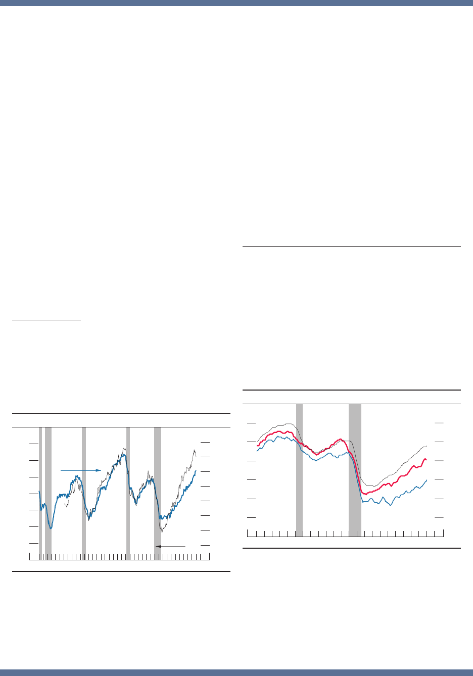
Domestic Developments
The labor market strengthened further
during the second half of 2017 and early
this year
Payroll employment has continued to post
solid gains, averaging 182,000 per month
in the seven months starting in July2017,
about the same pace as in the rst half of
2017.
2
Although net job creation last year was
slightly slower than in 2016, it has remained
considerably faster than what is needed, on
average, to absorb new entrants to the labor
force and is therefore consistent with the
view that the labor market has strengthened
further (gure1). The strength of the labor
market is also evident in the decline in the
unemployment rate to 4.1percent in January,
¼percentage point below its level in June2017
and about ½percentage point below the
median of Federal Open Market Committee
(FOMC) participants’ estimates of its longer-
run normal level (gure2).
Other indicators also suggest that labor
market conditions have continued to tighten.
The labor force participation rate (LFPR)—
that is, the share of adults either working or
actively looking for work—was 62.7percent
in January. The LFPR is little changed, on
net, since early 2014 (gure3). However, the
average age of the population is continuing
to increase. In particular, the members of the
baby-boom cohort increasingly are moving
into their retirement years, a time when labor
force participation typically is low. That
development implies that a sustained period
in which the demand for and supply of labor
were in balance would be associated with a
downward trend in the overall participation
rate. Accordingly, the at prole of the LFPR
2. The hurricanes that struck the United States during
the second half of last year caused substantial variation
in the month-to-month pattern of job gains, but the
average performance over the period as a whole was
probably substantially unaected.
during the past few years is consistent with
an overall picture of improving labor market
conditions. In line with this perspective, the
LFPR for individuals aged 25 to 54—which is
much less sensitive to population aging—has
been rising since 2015. The employment-
to-population ratio for individuals 16 and
older—that is, the share of people who are
working—was 60.1percent in January and has
been increasing since 2011; this gain primarily
reects the decline in the unemployment rate.
(The box “How Tight Is the Labor Market?”
describes the available measures of labor
market slack in more detail.)
Other indicators are also consistent with
continuing strong labor demand. The
number of people ling initial claims for
unemployment insurance has remained near
its lowest level in decades.
3
As reported in the
Job Openings and Labor Turnover Survey, the
rate of job openings remained elevated in the
second half of 2017, while the rate of layos
remained low. In addition, the rate of quits
stayed high, an indication that workers are able
to obtain a new job when they seek one.
3. Initial claims jumped in the fall of 2017 as a
consequence of disruptions from the hurricanes and then
returned to a low level.
Total nonfarm
800
600
400
200
+
_
0
200
400
Thousands of jobs
2018201720162015201420132012201120102009
1. Net change in payroll employment
3-month moving averages
Private
S
OURCE
: Bureau of Labor Statistics via Haver Analytics.
Part 1
recent economic and financiaL deveLoPments
6 PART 1: RECENT ECONOMIC AND FINANCIAL DEVELOPMENTS
Employment-to-population ratio
Prime-age labor force participation rate
56
58
60
62
64
66
68
Percent
80
81
82
83
84
85
20182014201020062002
3. Labor force participation rates and
employment-to-population ratio
Percent
Labor force participation rate
NOTE
: The data are monthly. The prime-age labor force participation
rate
is a percentage of the population aged 25 to 54. The labor force
participation
rate and the employment-to-population ratio are percentages of the
population
aged 16 and over.
S
OURCE
: Bureau of Labor Statistics via Haver Analytics.
Unemployment rates have declined across
demographic groups, but unemployment
remains high for some groups
Unemployment rates have trended downward
across racial and ethnic groups (gure4). The
decline in the unemployment rate for blacks or
African Americans over the past few years has
been particularly notable. This broad pattern
is typical: The unemployment rates for blacks
and Hispanics tend to rise considerably more
than the rates for whites and Asians during
recessions, and then they decline more rapidly
during expansions. Yet even with the recent
narrowing, the disparities in unemployment
rates across demographic groups remain
substantial and largely the same as before the
recession. The unemployment rate for whites
has averaged 3.7percent since the middle of
2017 and the rate for Asians has been about
3.3percent, while the unemployment rates for
Hispanics or Latinos (5.0percent) and blacks
(7.3percent) have been substantially higher.
In addition, the labor force participation
rates for blacks, Hispanics, and Asians have
generally been lower than those for whites
of the same age group. As the labor market
U-5
U-4
U-6
4
6
8
10
12
14
16
18
Percent
2018201620142012201020082006
2. Measures of labor underutilization
Monthly
Unemployment rate
N
OTE: Unemployment rate measures total unemployed as a percentage of the labor force. U-4 measures total unemployed plus discouraged workers, as a
percentage of the labor force plus discouraged workers. Discouraged workers are a subset of marginally attached workers who are not currently looking for work
because they believe no jobs are available for them. U-5 measures total unemployed plus all marginally attached to the labor force, as a percentage of the labor
force plus persons marginally attached to the labor force. Marginally attached workers are not in the labor force, want and are
available for work, and have looked
for a job in the past 12 months. U-6 measures total unemployed plus all marginally attached workers plus total employed part time for economic reasons, as a
percentage of the labor force plus all marginally attached workers. The shaded bar indicates a period of business recession as defined by the National Bureau of
Economic Research.
S
OURCE
: Bureau of Labor Statistics via Haver Analytics.
MONETARY POLICY REPORT: FEBRUARY 2018 7
has strengthened over the past few years, the
participation rates for prime-age individuals in
each of these groups have risen.
Growth of labor compensation has been
moderate . . .
Despite the strong labor market, the available
indicators generally suggest that the growth
of hourly compensation has been moderate.
Growth of compensation per hour in the
business sector—a broad-based measure
of wages, salaries, and benets that is quite
volatile—was 2¼percent over the four
quarters ending in 2017:Q4 (gure5), well
above the low reading in 2016 but about in
line with the average annual increase from
2010 to 2015.
4
The employment cost index—
which also measures both wages and the cost
to employers of providing benets—was up
about 2½percent in the fourth quarter of
2017 relative to its year-ago level, roughly
4. The compensation per hour measure of wages and
salaries declined at the end of 2016, possibly reecting
the shifting of bonuses or other types of income into
2017 in anticipation of a possible cut in personal income
tax rates.
Black or African American
Asian
Hispanic or Latino
2
4
6
8
10
12
14
16
18
Percent
2018201620142012201020082006
4. Unemployment rate by race and ethnicity
Monthly
White
N
OTE: Unemployment rate measures total unemployed as a percentage of the labor force. Persons whose ethnicity is identified as Hispanic or Latino may be of
any race. The shaded bar indicates a period of business recession as defined by the National Bureau of Economic Research.
S
OURCE
: Bureau of Labor Statistics via Haver Analytics.
Employment cost index
Atlanta Fed's Wage Growth Tracker
Average hourly earnings
1
+
_
0
1
2
3
4
5
6
Percent change from year earlier
20182016201420122010
5. Measures of change in hourly compensation
Compensation per hour,
business sector
N
OTE: Business-sector compensation is on a four-quarter
percentage
change basis. For the employment cost index, change is over the 12
months
ending in the last month of each quarter; for average hourly earnings,
change
is from 12 months earlier; for the Atlanta Fed's Wage Growth Tracker,
the
data are shown as a 3-month moving average of the 12-month
percent
change.
S
OURCE
: Bureau of Labor Statistics via Haver Analytics; Federal
Reserve
Bank of Atlanta, Wage Growth Tracker.
8 PART 1: RECENT ECONOMIC AND FINANCIAL DEVELOPMENTS
The fact that the LFPR for prime-age men remains
below its pre-recession levels might suggest that slack
remains along this dimension; however, the lower
level of the LFPR for prime-age men primarily seems
to reect the continuation of a decades-long secular
decline rather than a cyclical shortfall in their LFPR. In
addition, the U-6 measure of labor utilization—which
includes the unemployed, those marginally attached
to the labor force, and those employed part time who
would like full-time work—rose even more steeply
than the unemployment rate during and immediately
after the recession and has since recovered to near
its pre-recession level. Although there is substantial
uncertainty about the trends in each of the components
of U-6, its current level can be cautiously interpreted
as consistent with a labor market close to full
employment.
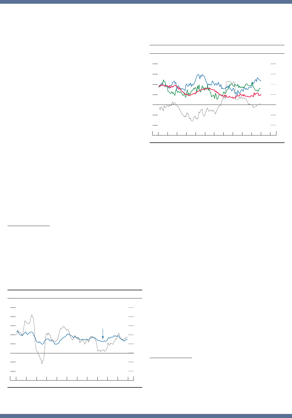
One can also look at less-direct indicators of labor
market tightness. For example, the share of small
businesses with at least one job opening that they view
as hard to ll is now close to its record levels in the late
1990s (as seen in the black line in gure B), consistent
with the notion that as the labor market tightens,
businesses nd it increasingly difcult to hire additional
workers. Similarly, survey measures of households’
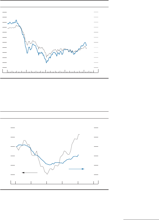
Any assessment of labor market tightness is
inherently uncertain, as it involves comparing current
labor market conditions with an estimate of conditions
that would prevail under full employment, where the
latter circumstance cannot be directly observed or
measured and can change over time. Many economists
would describe the labor market as being at full
employment when the unemployment rate has reached
an “equilibrium” level, sometimes called the natural
rate of unemployment or the longer-run normal rate of
unemployment. In judging the level of full employment,
one may also consider additional margins of labor
utilization—including the labor force participation rate
(LFPR), the share of workers employed part time who
would like to be working full time, and individuals
who are classied as marginally attached to the labor
force—as compared with trends in these measures.
While the uncertainty around the “normal” trends in
all of these variables is substantial, the labor market
in early 2018 appears to be near or a little beyond full
employment.
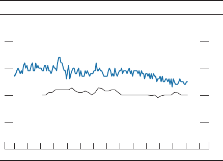
The unemployment rate is now somewhat below
most estimates of its natural rate. Specically, the
unemployment rate in January, at 4.1percent, is
½percentage point below the median of Federal Open
Market Committee (FOMC) participants’ estimates of
the longer-run normal rate of unemployment, which
was reported to have been 4.6percent as of the
December2017 FOMC meeting. The unemployment
rate is also about ½percentage point below the
Congressional Budget Ofce’s (CBO) current estimate
of the natural rate; by this measure, the labor market is
about as tight as it was in the late 1980s but less tight
than in the late 1990s (gure A). That said, the median
of FOMC participants’ estimates of the longer-run
normal rate of unemployment and the CBO’s estimate
of the natural rate of unemployment have both been
revised down by about 1percentage point over the past
few years, one indication of the substantial uncertainty
surrounding estimates of the “full employment” rate of
unemployment.
1
As discussed in the main text, the LFPR has been
roughly unchanged, on net, over the past four years,
representing an important cyclical improvement
relative to its declining trend. While estimates of the
trend LFPR are subject to substantial uncertainty and
differ among analysts, the current level of the LFPR
is relatively close to many estimates of its trend.
2
How Tight Is the Labor Market?
1. As another indication of this uncertainty, the range of
FOMC participants’ estimates of the longer-run normal rate of
unemployment was 4.3 to 5.0percent in December2017.
2. For a variety of approaches to assessing the level
of trend LFPR and the associated range of estimates, see
Stephanie Aaronson, Tomaz Cajner, Bruce Fallick, Felix
1
+
_
0
1
2
3
4
5
Percent of labor force
2017201320092005200119971993198919851981
A. Unemployment rate gap
Quarterly
NOTE
: The unemployment rate gap is the unemployment rate minus
the
Congressional
Budget Office's estimate of the natural rate of
unemployment.
The
shaded bars indicate periods of business recession as defined by
the
National Bureau of Economic Research.
SOURCE: For unemployment rate, Bureau of Labor Statistics; for
natural
rate of unemployment, Congressional Budget Office; all via Haver Analytics.
Galbis-Reig,Christopher Smith, and William Wascher (2014),
“Labor Force Participation: Recent Developments and
Future Prospects,” Brookings Papers on Economic Activity,
Fall, pp. 197–275, https://www.brookings.edu/wp-content/
uploads/2016/07/Fall2014BPEA_Aaronson_et_al.pdf.
Estimates of trend LFPR are also provided by the CBO in their
recurring publication The Budget and Economic Outlook and
its updates.
MONETARY POLICY REPORT: FEBRUARY 2018 9
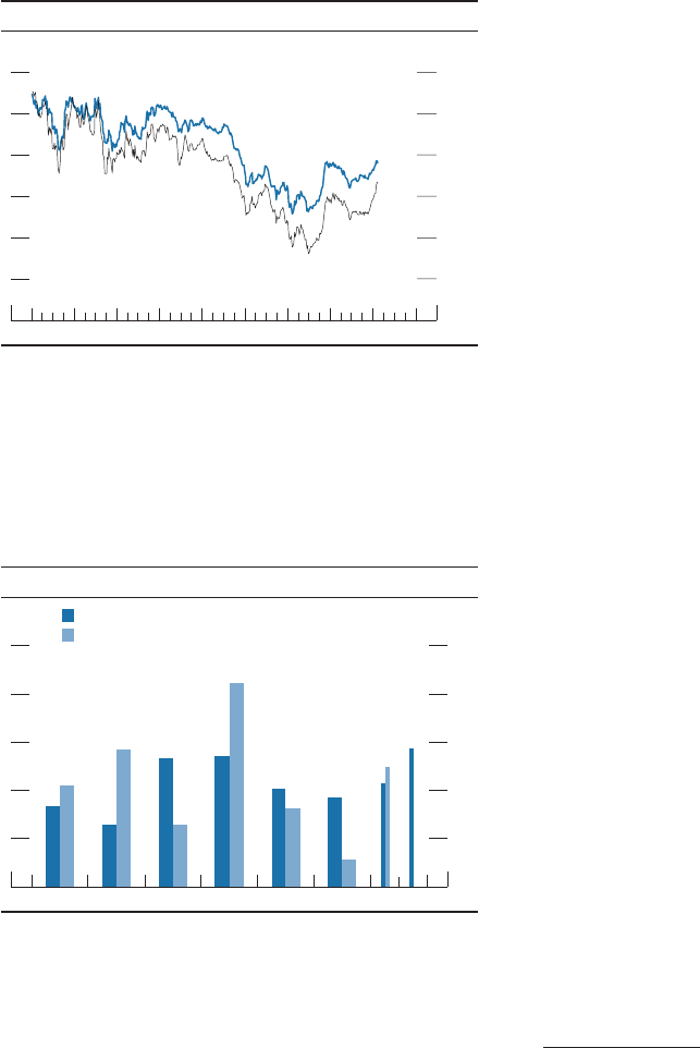
taken longer for businesses to nd workers in recent
years, yet wage growth has remained steady or slowed.
Finally, while the aggregate labor market appears
to be modestly tight at the moment, not all individuals
have beneted equally from these developments. As
discussed in the main text, noticeable differences
in labor market outcomes remain present across
racial and ethnic groups. Moreover, the labor market
improvement in recent years has not been sufcient
to make important progress in narrowing income
inequality. Finally, regional disparities are also striking,
and in certain aspects these disparities have widened
in recent years; for example, the employment-
to-population ratio for prime-age individuals has
recovered less for those outside of metro areas than for
those in metro areas (gure C).
5
perceptions about job availability are currently at high
levels, as shown by the blue line in gure B.
However, despite reports that employers are now
having more difculties nding qualied workers,
hiring has continued apace. Although payroll
employment gains have gradually slowed over time
from about 250,000 per month, on average, in 2014
to about 180,000 per month, on average, in 2017, job
growth remains consistent with further strengthening
in the labor market.
3
Finally, the pace of wage gains
has been moderate; while wage gains have likely been
held down by the sluggish pace of productivity growth
in recent years, serious labor shortages would probably
bring about larger increases than have been observed
thus far.
It is possible that labor shortages have arisen in
certain pockets of the economy, which could be an
early indication of bottlenecks that are not yet readily
apparent in the aggregate labor market. However, even
at the industry level it is difcult to see much evidence of
emerging supply constraints.
4
In some industries, such as
trade and transportation as well as leisure and hospitality,
employment growth has slowed markedly and it has
Job availability
20
40
60
80
100
120
140
160
Index
5
10
15
20
25
30
35
2018201420102006200219981994199019861982
B. Job availability and hard-to-fill positions
Percent
Hard-to-fill
N
OTE: Job availability is the proportion of households believing jobs
are
plentiful
minus the proportion believing jobs are hard to get, plus
100.
Hard-to-fill
is the three-month moving average of the percent of
small
businesses
surveyed with at least one hard-to-fill job opening, and it
is
seasonally adjusted by Federal Reserve Board staff. Monthly hard-to-fill data
from
the National Federation of Independent Business start in January
1986.
The
shaded bars indicate periods of business recession as defined by
the
National Bureau of Economic Research. Data are monthly.
SOURCE
: For job availability, Conference Board; for hard-to-fill,
National
Federation of Independent Business.
3. Payroll gains in the range of about 90,000 to 120,000
per month are estimated to be consistent with a constant
unemployment rate and a decline in the labor force
participation rate in line with its demographically driven trend.
4. The analysis behind this statement considered six
broad industries—construction, manufacturing, trade and
Non-metro
Smaller MSAs
72
74
76
78
80
82
Percent
201820162014201220102008200620042002200019981996
C. Prime-age employment-to-population ratio by
metropolitan status
Monthly
Larger MSAs
N
OTE: The data are 12-month centered moving averages.
Larger
metropolitan statistical areas (MSAs) consist of 500,000 people or more,
and
smaller MSAs consist of 100,000 to 500,000 people. The shaded bars
indicate
periods of business recession as defined by the National Bureau of Economic
Research.
S
OURCE
: Alison Weingarden (2017), “Labor Market Outcomes
in
Metropolitan and Non-metropolitan Areas: Signs of Growing
Disparities,”
FEDS Notes (Washington: Board of Governors of the Federal
Reserve
System, September 25),
www.federalreserve.gov/econres/notes/feds-notes/
labor-market-outcomes-in-metropolitan-and-non-metropolitan-areas-signs-of
-growing-disparities-20170925.htm. Calculations use data from the
U.S.
Census Bureau, Current Population Survey; note that the Bureau of
Labor
Statistics is involved in the survey process for the Current Population Survey.
transportation, health and education, leisure and hospitality,
and professional and business services.
5. See Alison Weingarden (2017), “Labor Market Outcomes
in Metropolitan and Non-metropolitan Areas: Signs of
Growing Disparities,” FEDS Notes (Washington: Board of
Governors of the Federal Reserve System, September25),
https://www.federalreserve.gov/econres/notes/feds-notes/labor-
market-outcomes-in-metropolitan-and-non-metropolitan-
areas-signs-of-growing-disparities-20170925.htm.
10 PART 1: RECENT ECONOMIC AND FINANCIAL DEVELOPMENTS
½percentage point faster than its gain a year
earlier. Among measures that do not take
account of benets, average hourly earnings
rose slightly less than 3percent through
January of this year, a gain that was somewhat
faster than the average increase in the
preceding few years. Similarly, the measure
of wage growth computed by the Federal
Reserve Bank of Atlanta that tracks median
12-month wage growth of individuals
reporting to the Current Population Survey
showed an increase of about 3percent in
January, similar to its readings from the past
three years and above the average increase in
the preceding few years.
5
. . . and likely was restrained by slow
growth of labor productivity
These moderate rates of compensation gain
likely reect the osetting inuences of a
tightening labor market and persistently
weak productivity growth. Since 2008, labor
productivity has increased only a little more
than 1percent per year, on average, well
below the average pace from 1996 through
2007 and also below the gains in the 1974–95
period (gure6). Considerable debate remains
about the reasons for the general slowdown in
productivity growth and whether it will persist.
The slowdown may be partly attributable
to the sharp pullback in capital investment
during the most recent recession and the
relatively long period of modest growth
in investment that followed, but a reduced
pace of capital deepening can explain only
a portion of the step-down. Beyond that,
some economists think that more recent
technological advances, such as information
technology, have been less revolutionary than
earlier general-purpose technologies, such as
electricity and internal combustion. Others
have pointed to a slowdown in the speed at
which capital and labor are reallocated toward
their most productive uses, which is reected
in fewer business start-ups and a reduced
5. The Atlanta Fed’s measure diers from others in
that it measures the wage growth only of workers who
were employed both in the current survey month and
12months earlier.
1
2
3
4
Percent, annual rate
6. Change in business-sector output per hour
1948–
73
1974–
95
1996–
2000
2001–
07
2008–
present
NOTE
: Changes are measured from Q4 of the year immediately
preceding
the period through Q4 of the final year of the period. The final period
is
measured from 2007:Q4 through 2017:Q4.
S
OURCE
: Bureau of Labor Statistics via Haver Analytics.
MONETARY POLICY REPORT: FEBRUARY 2018 11
pace of hiring and investment by the most
innovative rms. Still others argue that there
have been important innovations in many
elds in recent years, from energy to medicine,
often underpinned by ongoing advances in
information technology, which augurs well for
productivity growth going forward. However,
those economists note that such productivity
gains may appear only slowly as new rms
emerge to exploit the new technologies and
as incumbent rms invest in new vintages of
capital and restructure their businesses.
Price ination remains below 2percent,
but the monthly readings picked up
toward the end of 2017
Consumer price ination, as measured by
the 12-month change in the price index for
personal consumption expenditures (PCE),
remained below the FOMC’s longer-run
objective of 2percent during most of 2017.
The PCE price index increased 1.7percent
over the 12 months ending in December2017,
about the same as in 2016 (gure7). Core
ination, which typically provides a better
indication than the headline measure of
where overall ination will be in the future,
was 1.5percent over the 12months ending in
December2017—0.4percentage point lower
than it had been one year earlier.
Both measures of ination reected some
weak readings in the spring and summer
of 2017. A portion of those weak readings
seemed attributable to idiosyncratic events,
such as a steep 1-month decline in the price
index for wireless telephone services. However,
the monthly readings on core ination were
somewhat higher during the last few months
of 2017, in contrast to the more typical pattern
that has prevailed in recent years in which
readings around the end of the year have
tended to be slightly below average. Moreover,
the 12-month change in the trimmed mean
PCE price index—an alternative indicator of
underlying ination produced by the Federal
Reserve Bank of Dallas that may be less
sensitive to idiosyncratic price movements—
was 1.7percent in December2017 and has
slowed by less than core PCE price ination
Excluding food
and energy
Trimmed mean
+
_
0
.5
1.0
1.5
2.0
2.5
3.0
12-month percent change
2017201620152014201320122011
7. Change in the price index for personal consumption
expenditures
Monthly
Total
NOTE
: The data extend through December 2017; changes are from one year
earlier.
SOURCE: For trimmed mean, Federal Reserve Bank of Dallas; for all else,
Bureau of Economic Analysis; all via Haver Analytics.
12 PART 1: RECENT ECONOMIC AND FINANCIAL DEVELOPMENTS
over the past 12 months.
6
(For more discussion
of ination both in the United States and
abroad, see the box “Low Ination in the
Advanced Economies.”)
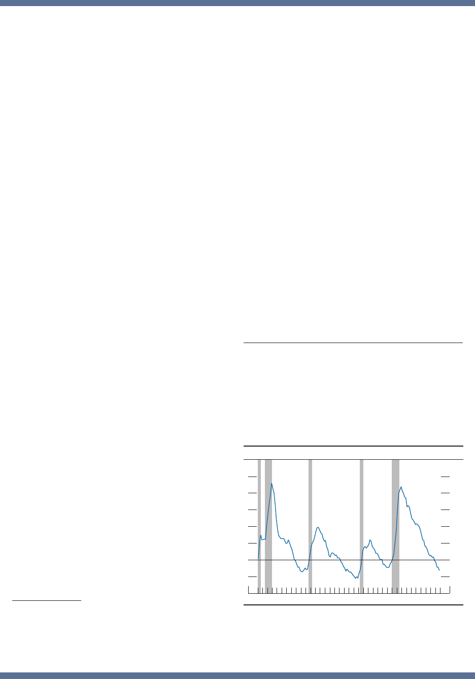
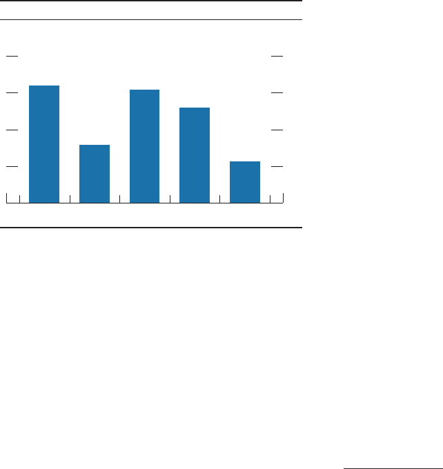
Oil and metals prices increased notably
Headline ination was a little higher than
core ination last year, which reected a rise
in consumer energy prices. The price of crude
oil rose from $48 per barrel at the end of June
to a peak of about $70 per barrel early in the
year and, even after recent declines, remains
more than 30percent above its mid-2017 level
(gure8). The upswing in oil prices appears to
have been driven primarily by strengthening
global demand as well as OPEC’s decision to
further extend its November2016 production
cuts through the end of 2018. The higher oil
prices fed through to moderate increases in the
cost of gasoline and heating oil.
Ination momentum was also supported by
nonfuel import prices, which rose throughout
2017 in part because of dollar depreciation
(gure9). That development marked a turn
from the past several years, during which
nonfuel import prices declined or held at.
In addition to the decline in the dollar,
nonfuel import prices were driven higher by a
substantial increase in the price of industrial
metals. Despite recent volatility, metals prices
remain higher, on net, boosted primarily by
improved prospects for global demand and
also by government policies that restrained
production in China.
In contrast, headline ination has been
held down by consumer food prices, which
increased only about ½percent in 2017 after
having declined in 2016. Food prices have
6. The trimmed mean index excludes whatever prices
showed the largest increases or decreases in a given
month; for example, the sharp decline in prices for
wireless telephone services in March2017 was excluded
from this index.
Spot price
20
30
40
50
60
70
80
90
100
110
120
130
Dollars per barrel
2014 2015 2016 2017 2018
8. Brent spot and futures prices
Weekly
24-month-ahead
futures contracts
N
OTE
: The data are weekly averages of daily data and extend
through
February 21, 2018.
S
OURCE: ICE Brent Futures via Bloomberg.
Nonfuel import prices
94
96
98
100
102
104
January 2014 = 100
70
80
90
100
110
120
20182017201620152014
9. Nonfuel import prices and industrial metals indexes
January 2014 = 100
Industrial metals
N
OTE
: The data for nonfuel import prices are monthly. The data for
industrial
metals are a monthly average of daily data and extend through
February 21, 2018.
S
OURCE
: For nonfuel import prices, Bureau of Labor Statistics; for
industrial
metals, S&P GSCI Industrial Metals Spot Index via Haver
Analytics.
MONETARY POLICY REPORT: FEBRUARY 2018 13
been restrained by softness in the prices of
farm commodities, which in turn has reected
robust supply in the United States and abroad.
Although the harvests for many crops in the
United States declined in 2017, they were
larger than had been expected earlier in
the year.
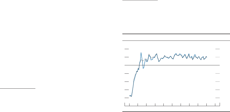
Survey-based measures of ination
expectations have been generally stable. . .
Expectations of ination likely inuence actual
ination by aecting wage- and price-setting
decisions. Survey-based measures of ination
expectations at medium- and longer-term
horizons have remained generally stable. In the
Survey of Professional Forecasters conducted
by the Federal Reserve Bank of Philadelphia,
the median expectation for the annual rate of
increase in the PCE price index over the next
10years has been around 2percent for the past
several years (gure10). In the University of
Michigan Surveys of Consumers, the median
value for ination expectations over the next
5 to 10years—which had drifted downward
starting in 2014—has held about at since the
end of 2016 at a level that is a few tenths lower
than had prevailed through 2014.
. . . and market-based measures of
ination compensation have increased in
recent months but remain relatively low
Ination expectations can also be gauged
by market-based measures of ination
compensation, though the inference is not
straightforward because market-based
measures can be importantly aected
by changes in premiums that provide
compensation for bearing ination and
liquidity risks. Measures of longer-term
ination compensation—derived either from
dierences between yields on nominal Treasury
securities and those on comparable Treasury
Ination-Protected Securities (TIPS) or from
ination swaps—have increased since June,
returning to levels seen in early 2017, but
Michigan survey expectations
for next 5 to 10 years
1
2
3
4
Percent
2018201620142012201020082006
SPF expectations
for next 10 years
10. Median inflation expectations
NOTE
: The Michigan survey data are monthly and extend
through
February; the February data are preliminary. The SPF data for
inflation
expectations for personal consumption expenditures are quarterly and
extend
from 2007:Q1 through 2018:Q1.
SOURCE: University of Michigan Surveys of Consumers; Federal
Reserve
Bank of Philadelphia, Survey of Professional Forecasters (SPF).
14 PART 1: RECENT ECONOMIC AND FINANCIAL DEVELOPMENTS
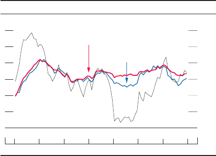
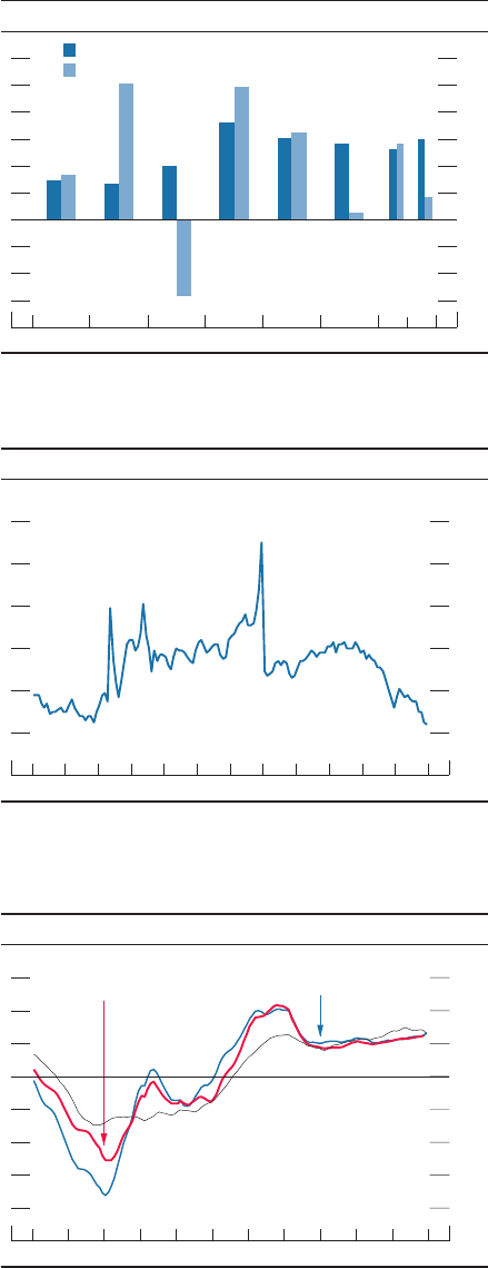
But our understanding of the forces that drive
ination is imperfect, and the fact that many advanced
economies are experiencing low ination at the same
time suggests that other, possibly more persistent,
factors may be at work. As one possibility, the natural
rate of unemployment—the rate at which labor markets
exert neither upward nor downward pressure on
ination—is highly uncertain, and it could be lower
in many economies than most economists estimate.
Alternatively, ination expectations could be lower
than suggested by the available indicators.
More-fundamental changes in the global economy
could also be contributing to the recent stretch of
lower ination. First, anecdotal reports suggest that
technological changes could be reducing pricing
power in many industries, holding down ination as
that occurs.
2
For example, the increased prevalence of
Internet shopping allows consumers to compare prices
more easily across sellers, possibly implying greater
competition that could be putting downward pressure
on consumer prices (gure C). While this hypothesis is
certainly plausible, it does not easily square with the
observation that, at least within the United States, prot
margins have been high (gure D).
3
Ination has been persistently low in recent years
across many advanced economies. In the United States,
both overall ination and core (excluding food and
energy prices) ination, as measured by the price index
for personal consumption expenditures, have run below
2percent for most of the period since 2008 (gureA).
In other advanced economies, measures of core
ination have run even lower in some cases, with core
ination in the euro area currently at around 1percent
and in Japan at close to zero (gure B).
What explains this period of low ination? Across
the advanced economies, the main factors holding
ination down likely include the extended period of
economic slack following the Great Recession and
the falling prices of oil and other commodities from
around mid-2014 to early 2016. In the United States,
ination also has been held down by the rise in the
foreign exchange value of the dollar from mid-2014
through 2016. The low core U.S. ination in 2017 has
been more of a puzzle (albeit modest in magnitude)
and harder to associate with an identiable cause.
1
As is discussed in the December2017 Summary of
Economic Projections (Part 3 of this report), most
Federal Reserve policymakers view these recent low
ination readings as likely to prove transitory and
project U.S. ination this year to move closer to their
2percent objective. Many private forecasters appear to
share this view.
Low Ination in the Advanced Economies
Excluding food
and energy
2
1
+
_
0
1
2
3
4
5
12-month percent change
201720152013201120092007
A. Change in the price index for personal consumption
expenditures
Monthly
Total
NOTE
: The data extend through December 2017; changes are from one year
earlier.
S
OURCE: Bureau of Economic Analysis via Haver Analytics.
1. For additional discussion of the reasons for low ination
in the United States, see Janet Yellen (2017), “Ination,
Uncertainty, and Monetary Policy,” speech delivered at
“Prospects for Growth: Reassessing the Fundamentals,” 59th
Annual Meeting of the National Association for Business
Economics, Cleveland, Ohio, September26, https://www.
federalreserve.gov/newsevents/speech/yellen20170926a.htm.
United Kingdom
Canada
Euro area
2
1
+
_
0
1
2
3
4
12-month percent change
201820162014201220102008
B. Inflation excluding food and energy in selected
advanced foreign economies
Monthly
Japan
N
OTE:
The data for the euro area incorporate the flash estimate for January
2018. The data for Canada and Japan extend through December 2017.
SOURCE:
For the United Kingdom, Office for National Statistics; for Japan,
Ministry
of International Affairs and Communications; for the euro
area,
Statistical
Office of the European Communities; for Canada,
Statistics
Canada; all via Haver Analytics.
2. Goldman Sachs (2017), “The Amazon Effect in
Perspective,” U.S. Economics Analyst (New York: Goldman
Sachs, September30).
3. See Council of Economic Advisers (2016), “Benets
of Competition and Indicators of Market Power,” Council
of Economic Advisers Issue Brief (Washington: CEA, April),
https://obamawhitehouse.archives.gov/sites/default/les/page/
les/20160414_cea_competition_issue_brief.pdf.

MONETARY POLICY REPORT: FEBRUARY 2018 15
than other consumers.
6
Others have pointed to a
slowdown in medical services price increases across
countries, possibly associated with either health-care
reform or scal austerity.
7
This slowdown has had a
material effect on U.S. ination, though the extent to
which these declines will persist is uncertain.
In summary, while standard economic models
appear to explain much of the post–Great Recession
period of low ination, they do not preclude other
explanations. Even as most policymakers expect
ination in their economies to move back to their
targets over time, they remain attentive to the possibility
that factors not included in those models, such as those
described here, may keep ination low. At the same
time, they are attentive to the opposite risk of ination
moving undesirably high, should tightening demand
conditions lead to faster rises in wages and prices than
currently anticipated.
Second, some observers have pointed to global
developments as helping to explain persistent low
ination across countries. These developments
include economic slack abroad or the integration of
emerging economies into the world economy, leading
to increased competition or downward pressures on
wages.
4
But the evidence that global slack can help
explain ination in a given country, beyond its effect
on commodity and import prices, is mixed at best.
5
Moreover, measures of integration, such as global
trade as a fraction of gross domestic product or the
participation in global value chains, appear to have
leveled off in recent years.
A number of other explanations for low global
ination have been advanced as well. These
explanations include some tentative evidence
suggesting that the aging of the population could be
exerting downward pressure on trend ination, perhaps
because retirees may tend to be more price conscious
0
1
2
3
4
5
6
7
8
9
10
Percent
2017201420112008200520021999
C. E-commerce sales as a share of retail sales
Quarterly
NOTE: E-commerce sales are sales of goods and services where an order
is
placed
by the buyer or where the price and terms of sale are negotiated
over
an online system. Payment may or may not be made online.
S
OURCE: Retail Indicators Branch, U.S. Census Bureau.
6
8
10
12
14
Percent
20172012200720021997199219871982
Quarterly
D. Corporate profits as a share of gross national product
NOTE: The data extend through 2017:Q3. Corporate profits
include
inventory valuation and capital consumption adjustments.
S
OURCE: Bureau of Economic Analysis via Haver Analytics.
4. See Claudio Borio and Andrew Filardo (2007),
“Globalisation and Ination: New Cross-Country Evidence
on the Global Determinants of Domestic Ination,” BIS
Working Papers 227 (Basel, Switzerland: Bank for International
Settlements, May), www.bis.org/publ/work227.pdf; and
Raphael Auer, Claudio Borio, and Andrew Filardo (2017), “The
Globalisation of Ination: The Growing Importance of Global
Value Chains,” BIS Working Papers 602 (Basel, Switzerland:
Bank for International Settlements, January), www.bis.org/
publ/work602.pdf.
5. See Jane Ihrig, Steven B. Kamin, Deborah Lindner,
and Jaime Marquez (2010), “Some Simple Tests of the
Globalization and Ination Hypothesis,” International Finance,
vol. 13 (Winter), pp. 343–75; and European Central Bank
(2017), “Domestic and Global Drivers of Ination in the Euro
Area,” ECB Economic Bulletin, no. 4 (June), pp. 72–96, https://
www.ecb.europa.eu/pub/pdf/other/ebart201704_01.en.pdf.
6. See Jong-Won Yoon, Jinill Kim, and Jungjin Lee (2014),
“Impact of Demographic Changes on Ination and the
Macroeconomy,” IMF Working Paper WP/14/210 (Washington:
International Monetary Fund, November), https://www.imf.
org/external/pubs/ft/wp/2014/wp14210.pdf. However, other
evidence suggests increased inationary pressure from an
aging population; see Mikael Juselius and Előd Takáts (2015),
“Can Demography Affect Ination and Monetary Policy?” BIS
Working Papers 485 (Basel, Switzerland: Bank for International
Settlements, February), https://www.bis.org/publ/work485.pdf.
7. See Tim Mahedy and Adam Shapiro (2017), “What’s
Down with Ination?” FRBSF Economic Letter 2017-35 (San
Francisco: Federal Reserve Bank of San Francisco, November),
https://www.frbsf.org/economic-research/publications/
economic-letter/2017/november/contribution-to-low-pce-
ination-from-healthcare); and Goldman Sachs (2017), “What
Can We Learn from Lower Ination Abroad?” U.S. Economics
Analyst (New York: Goldman Sachs, November12)
16 PART 1: RECENT ECONOMIC AND FINANCIAL DEVELOPMENTS
nevertheless remain relatively low (gure11).
7
The TIPS-based measure of 5-to-10-year-
forward ination compensation and the
analogous measure of ination swaps are now
slightly lower than 2¼percent and 2½percent,
respectively, with both measures below the
ranges that persisted for most of the 10years
before the start of the notable declines
in mid-2014.
Real gross domestic product growth
picked up in the second half of 2017
Real gross domestic product (GDP) is
reported to have risen at an annual rate of
nearly 3percent in the second half of 2017
after increasing slightly more than 2percent
in the rst half of 2017 (gure12). Much of
that faster growth reects the stabilization
of inventory investment, which had slowed
considerably in the rst half of last year.
Private domestic nal purchases—that is,
nal purchases by U.S. households and
businesses, which tend to provide a better
indication of future GDP growth than most
other components of overall spending—rose
at a solid annual rate of about 3½percent in
the second half of the year, similar to the rst-
half pace.
The economic expansion continues to
be supported by steady job gains, rising
household wealth, favorable consumer
sentiment, strong economic growth abroad,
and accommodative nancial conditions,
including the still low cost of borrowing and
easy access to credit for many households and
businesses. In addition to these factors, very
7. Ination compensation implied by the TIPS
breakeven ination rate is based on the dierence, at
comparable maturities, between yields on nominal
Treasury securities and yields on TIPS, which are indexed
to the headline consumer price index (CPI). Ination
swaps are contracts in which one party makes payments
of certain xed nominal amounts in exchange for cash
ows that are indexed to cumulative CPI ination over
some horizon. Focusing on ination compensation 5 to
10years ahead is useful, particularly for monetary policy,
because such forward measures encompass market
participants’ views about where ination will settle in the
long term after developments inuencing ination in the
short term have run their course.
1
2
3
4
5
Percent, annual rate
2017201620152014201320122011
12. Change in real gross domestic product and gross
domestic income
H1
H2*
*Gross domestic income is not yet available for 2017:H2.
SOURCE: Bureau of Economic Analysis via Haver Analytics.
Gross domestic product
Gross domestic income
Inflation swaps
1.0
1.5
2.0
2.5
3.0
3.5
Percent
20182016201420122010
11. 5-to-10-year-forward inflation compensation
Weekly
TIPS breakeven rates
N
OTE
:The data are weekly averages of daily data and extend
through
February 16, 2018. TIPS is Treasury Inflation-Protected Securities.
SOURCE: Federal Reserve Bank of New York; Barclays; Federal
Reserve
Board staff estimates.
MONETARY POLICY REPORT: FEBRUARY 2018 17
upbeat business sentiment appears to have
supported solid growth over the past year.
Ongoing improvement in the labor
market and gains in wealth continue to
support consumer spending . . .
Supported by ongoing improvement in the
labor market, real consumer spending rose at
a solid annual rate of 3percent in the second
half of 2017, a somewhat faster pace than
in the rst half. Real disposable personal
income—that is, income after taxes and
adjusted for price changes—increased at a
modest average rate of 1percent in 2016 and
2017, as real wages changed little over this
period (gure13). With spending growth
estimated to have outpaced income growth, the
personal saving rate has declined considerably
since the end of 2015 (gure14).
Consumer spending has also been supported
by further increases in household net wealth.
Broad measures of U.S. equity prices rose
robustly last year, though markets have been
volatile in recent weeks; house prices have also
continued to climb, strengthening the wealth
of homeowners (gure15). As a result of the
increases in home and equity prices, aggregate
household net worth rose appreciably in 2017.
In fact, at the end of the third quarter of 2017,
household net worth was 6.7 times the value of
disposable income, the highest-ever reading for
that ratio, which dates back to 1947 (gure16).
. . . borrowing conditions for consumers
remain generally favorable . . .
Consumer credit expanded in 2017 at about
the same pace as in 2016 (gure17). Financing
conditions for most types of consumer loans
are generally favorable. However, banks have
continued to tighten standards on credit card
and auto loans for borrowers with low credit
scores, possibly in response to some upward
drift in delinquency rates for those borrowers.
Mortgage credit has remained readily available
for households with solid credit proles, but
it was still dicult to access for households
with low credit scores or harder-to-document
incomes.
3
2
1
+
_
0
1
2
3
4
5
6
Percent, annual rate
2017201620152014201320122011
13. Change in real personal consumption expenditures
and disposable personal income
H1
H2
SOURCE
: Bureau of Economic Analysis via Haver Analytics.
Personal consumption expenditures
Disposable personal income
2
4
6
8
10
12
PercentMonthly
201720152013201120092007
14. Personal saving rate
NOTE: Data are through December 2017.
SOURCE
: Bureau of Economic Analysis via Haver Analytics.
CoreLogic
price index
S&P/Case-Shiller
national index
20
15
10
5
+
_
0
5
10
15
Percent change from year earlier
201720152013201120092007
15. Prices of existing single-family houses
Monthly
Zillow index
N
OTE
: The data for the S&P/Case-Shiller index extend through November
2017.
The data for the Zillow index and the CoreLogic index extend through
December 2017.
SOURCE
: CoreLogic Home Price Index; Zillow; S&P/Case-Shiller U.S.
National Home Price Index. The S&P/Case-Shiller Index is a product of S&P
Dow
Jones Indices LLC and/or its affiliates. (For Dow Jones Indices
licensing information, see the note on the Contents page.)
18 PART 1: RECENT ECONOMIC AND FINANCIAL DEVELOPMENTS
Although household borrowing continued to
increase last year, the household debt service
burden—the ratio of required principal and
interest payments on outstanding household
debt to disposable income, measured for the
household sector as a whole—remained low by
historical standards.
. . . and consumer condence is strong
Consumers have remained optimistic about
their economic situation. As measured by the
Michigan survey, consumer sentiment was
solid throughout 2017, likely reecting rising
income, job gains, and low ination (gure18).
Furthermore, the share of households
expecting real income to rise over the next year
or two has continued to strengthen and now
exceeds its pre-recession level.
Activity in the housing sector has
improved modestly
Real residential investment spending increased
around 2percent in 2017, about the same
modest gain that was seen in 2016. Housing
activity was soft in the spring and summer,
possibly reecting the rise in mortgage interest
rates early in the year, and then picked up
toward the end of the year. For the year as a
whole, sales of new and existing homes gained,
and single-family housing starts increased
(gures 19 and 20). In contrast, multifamily
housing starts continued to edge down from
the solid pace seen in 2016. Going forward,
lean inventories are likely to support further
gains in homebuilding activity, as the months’
supply of homes for sale has remained near
low levels.
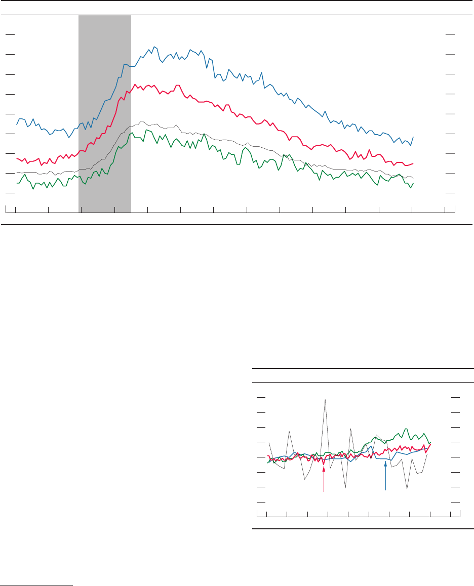
Business investment has continued to
rebound . . .
Real outlays for business investment—that
is, private nonresidential xed investment—
rose at an annual rate of about 6percent
in the second half of 2017, a bit below the
gain in the rst half but still notably faster
than the unusually weak pace recorded
in 2016 (gure21). Business spending on
equipment and intangibles (such as research
Consumer sentiment
50
60
70
80
90
100
110
Index
50
60
70
80
90
2018201620142012201020082006
Diffusion index
18. Indexes of consumer sentiment and income expectations
Real income expectations
N
OTE
: The data extend through February 2018; the February data are
preliminary. The consumer sentiment data are monthly and are indexed to
100 in 1966. The real income expectations data are calculated as the net
percentage of survey respondents expecting family income to go up more
than prices during the next year or two plus 100 and are shown as a
three-month moving average.
S
OURCE
: University of Michigan Surveys of Consumers.
200
+
_
0
200
400
600
800
1,000
Billions of dollars, annual rate
201720152013201120092007
17. Changes in household debt
Sum
NOTE
: The values for 2017 are the averages of the seasonally
adjusted
annualized quarterly flows through 2017:Q3.
S
OURCE: Federal Reserve Board, Statistical Release Z.1,
“Financial
Accounts of the United States.”
Mortgages
Consumer credit
5.0
5.5
6.0
6.5
7.0
Ratio
20172014201120082005200219991996
16. Wealth-to-income ratio
Quarterly
NOTE
: The data extend through 2017:Q3. The series is the ratio of
household net worth to disposable personal income.
SOURCE: For net worth, Federal Reserve Board, Statistical Release Z.1,
“Financial
Accounts of the United States”; for income, Bureau of Economic
Analysis via Haver Analytics.
MONETARY POLICY REPORT: FEBRUARY 2018 19
and development) advanced at a solid pace
in the second half of the year, and forward-
looking indicators of business spending are
generally favorable: Orders and shipments of
capital goods have posted net gains in recent
months, and indicators of business sentiment
and activity remain very upbeat. That said,
business outlays on structures turned down in
the second half of 2017, as investment growth
in drilling and mining structures retreated
from a very rapid pace in the rst half and
investment in other nonresidential structures
declined.
. . . while corporate nancing conditions
have remained accommodative
Aggregate ows of credit to large nonnancial
rms remained solid through the third
quarter, supported in part by continued low
interest rates (gure22). The gross issuance
of corporate bonds stayed robust during
the second half of 2017, and yields on both
investment-grade and high-yield corporate
bonds remained low by historical standards
(gure23).
Despite solid growth in business investment,
outstanding commercial and industrial (C&I)
loans on banks’ books continued to rise
only modestly in the third quarter of 2017.
Respondents to the Senior Loan Ocer
Opinion Survey on Bank Lending Practices,
or SLOOS, reported that demand for C&I
loans declined in the third quarter and was
little changed in the fourth quarter even as
lending standards and terms on such loans
eased.
8
Respondents attributed this decline in
demand in part to rms drawing on internally
generated funds or using alternative sources
of nancing. Financing conditions for small
businesses appear to have remained favorable,
and although credit growth has remained
sluggish, survey data suggest this sluggishness
is largely due to continued weak demand for
credit by small businesses.
8. The SLOOS is available on the Board’s website at
https://www.federalreserve.gov/data/sloos/sloos.htm.
Existing home sales
.2
.4
.6
.8
1.0
1.2
1.4
1.6
Millions, annual rate
3.0
3.5
4.0
4.5
5.0
5.5
6.0
6.5
7.0
7.5
2018201620142012201020082006
19. New and existing home sales
Millions, annual rate
New home sales
N
OTE
: Data are monthly. New home sales extend through December
2017
and include only single-family sales. Existing home sales
includes
single-family, condo, townhome, and co-op sales.
S
OURCE
: For new home sales, U.S. Census Bureau; for existing
home
sales, National Association of Realtors; all via Haver Analytics.
10
5
+
_
0
5
10
15
Percent, annual rate
20172016201520142013201220112010
21. Change in real private nonresidential fixed investment
H1
H2
SOURCE
: Bureau of Economic Analysis via Haver Analytics.
Structures
Equipment and intangible capital
Multifamily starts
Single-family permits
0
.4
.8
1.2
1.6
2.0
Millions of units, annual rate
2018201620142012201020082006
20. Private housing starts and permits
Monthly
Single-family starts
SOURCE: U.S. Census Bureau via Haver Analytics.
20 PART 1: RECENT ECONOMIC AND FINANCIAL DEVELOPMENTS
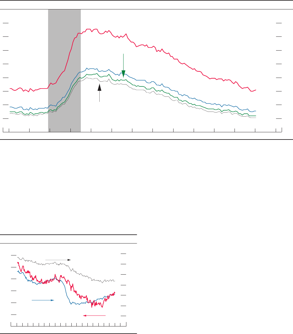
Net exports subtracted from GDP
growth in the fourth quarter after
providing a modest addition during the
rest of the year
U.S. real exports expanded at a moderate
pace in the second half of last year after
having increased more rapidly in the rst half,
supported by solid foreign growth (gure24).
At the same time, real imports surged in the
fourth quarter following a slight contraction in
the third quarter. As a result, real net exports
moved from modestly lifting U.S. real GDP
growth during the rst three quarters of 2017
to subtracting more than 1percentage point in
the fourth quarter. Although the nominal trade
and current account decits narrowed in the
third quarter of 2017, the trade decit widened
in the fourth quarter (gure25).
Federal scal policy actions had a
roughly neutral effect on economic
growth in 2017 . . .
Federal government purchases rose 1percent
in 2017, and policy actions had little eect on
federal taxes or transfers (gure26). Under
currently enacted legislation, which includes
the Tax Cuts and Jobs Act (TCJA) and the
Bipartisan Budget Act, federal scal policy
will likely provide a moderate boost to GDP
growth this year.
9
The federal unied decit continued to widen
in scal year 2017, reaching 3½percent of
nominal GDP. Although expenditures as a
share of GDP were relatively stable at a little
under 21percent, receipts moved lower in 2017
to roughly 17percent of GDP (gure27).
The ratio of federal debt held by the public
to nominal GDP was 75¼percent at the end
of scal year 2017 and remains quite elevated
relative to historical norms (gure28).
9. The Joint Committee on Taxation estimates that the
TCJA will reduce average annual tax revenue by a little
more than 1percent of GDP over the next few years.
This revenue estimate does not account for the potential
macroeconomic eects of the legislation.
3
+
_
0
3
6
9
12
15
Percent, annual rate
2017201620152014
24. Change in real imports and exports of goods
and services
H1
Q3
Q4
S
OURCE
: Bureau of Economic Analysis via Haver Analytics.
Imports
Exports
Double-A
High-yield
0
2
4
6
8
10
12
14
16
18
20
Percentage points
2000 2003 2006 2009 2012 2015 2018
23. Corporate bond yields, by securities rating
Daily
Triple-B
N
OTE: The yields shown are yields on 10-year bonds.
S
OURCE
: ICE Bank of America Merrill Lynch Indices, used
with
permission.
40
20
+
_
0
20
40
60
80
Billions of dollars, monthly rate
201720152013201120092007
22. Selected components of net debt financing for
nonfinancial businesses
Sum
Q3
H1
S
OURCE
: Federal Reserve Board, Statistical Release Z.1,
“Financial
Accounts of the United States.”
Commercial paper
Bonds
Bank loans
MONETARY POLICY REPORT: FEBRUARY 2018 21
. . . and the scal position of most state
and local governments is stable
The scal position of most state and local
governments is stable, although there is a
range of experiences across these governments.
Many state governments are experiencing
lackluster revenue growth, as income tax
collections have only edged up, on average,
in recent quarters. In contrast, house price
gains have continued to push up property tax
revenues at the local level. Employment in the
state and local government sector only inched
up in 2017, while outlays for construction by
these governments continued to decline on net
(gure29).
Financial Developments
The expected path of the federal funds
rate has moved up
The path of the expected federal funds rate
implied by market quotes on interest rate
derivatives has moved up on net since the
middle of last year amid an improving global
growth outlook (gure30). Part of the upward
shift occurred around FOMC communications
in the fall that were interpreted as implying a
somewhat quicker pace of policy rate increases
than had been previously anticipated. The
expected policy path also moved higher around
the time when the U.S. tax legislation was
nalized.
Survey-based measures of the expected path
of the policy rate have been generally little
changed on net, suggesting that part of the
rise in the market-implied path reected higher
term premiums. In the Federal Reserve Bank
of New York’s Survey of Primary Dealers and
Survey of Market Participants, which were
conducted just before the January2018 FOMC
meeting, the median respondents expected
three 25 basis point increases in the FOMC’s
target range for the federal funds rate as the
most likely outcome for this year, unchanged
from what they had expected in surveys
conducted before the June FOMC meeting.
Market-based measures of uncertainty about
Expenditures
14
16
18
20
22
24
26
Percent of nominal GDPPercent of nominal GDP
201720132009200520011997
Annual
27. Federal receipts and expenditures
Receipts
N
OTE
: The receipts and expenditures data are on a unified-budget basis
and
are
for fiscal years (October through September); gross domestic
product
(GDP) data are for the four quarters ending in Q4.
S
OURCE
: Office of Management and Budget via Haver Analytics.
8
6
4
2
+
_
0
2
4
6
Percent, annual rate
201720162015201420132012201120102009
26. Change in real government expenditures on
consumption and investment
H1
H2
SOURCE: Bureau of Economic Analysis via Haver Analytics.
Federal
State and local
Current account
7
6
5
4
3
2
1
+
_
0
Percent of nominal GDP
201720152013201120092007200520032001
25. U.S. trade and current account balances
Quarterly
Trade
N
OTE: GDP is gross domestic product. Current account data
extend
through 2017:Q3.
SOURCE: Bureau of Economic Analysis via Haver Analytics.
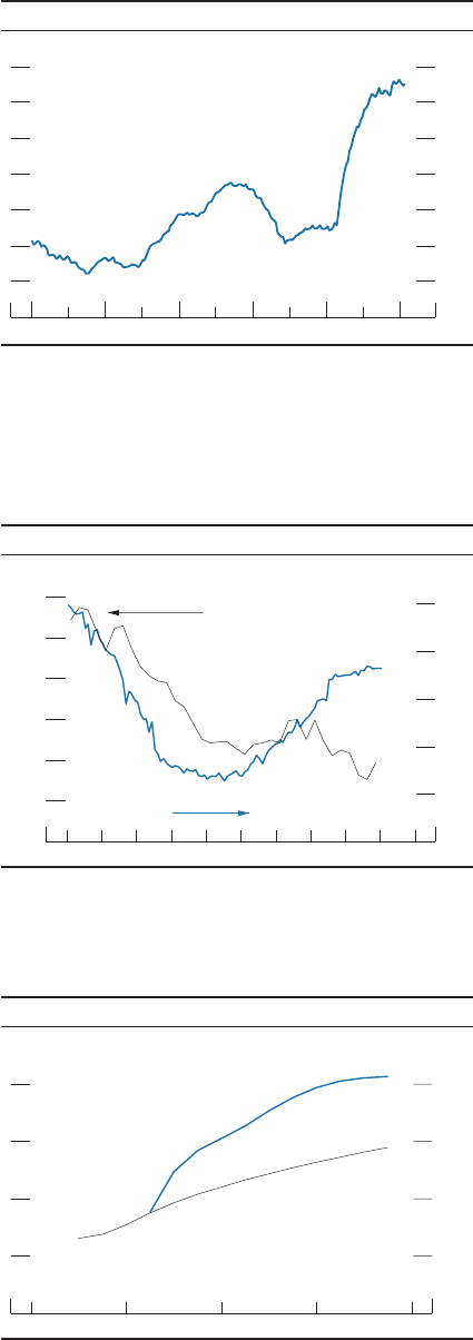
22 PART 1: RECENT ECONOMIC AND FINANCIAL DEVELOPMENTS
the policy rate approximately one to two years
ahead have, on balance, edged up from their
levels in the middle of 2017.
The nominal Treasury yield curve has
shifted up
The nominal Treasury yield curve has shifted
up on net since the middle of 2017, owing
to greater optimism about the global growth
outlook and investors’ perceptions of higher
odds for the removal of monetary policy
accommodation (gure31). Yields on shorter-
term nominal Treasury securities increased
relatively more than those on longer-term
nominal Treasury securities, thus resulting in
some attening of the yield curve. According
to market participants, among the factors
contributing to this outcome has been the
Treasury Department’s stated intention to
increase its reliance on issuance of short-dated
securities, as discussed in the two most recent
releases of the Treasury’s quarterly nancing
statement.
Consistent with the changes in Treasury yields,
yields on 30-year agency mortgage-backed
securities (MBS)—an important determinant
of mortgage interest rates—increased but
remain quite low by historical standards
(gure32).
Broad equity price indexes have
increased further . . .
Broad U.S. equity indexes, despite some
declines seen in recent weeks, have, on balance,
increased further since June2017, with most
of the net gains occurring during the nal
quarter of last year (gure33). Equity prices
were reportedly supported in part by an
increase in investors’ condence that changes
to the federal tax law will boost corporate
earnings. Stock prices generally increased
across industries outside utilities and real
estate, two sectors for which the increases in
interest rates described earlier are likely to have
weighed more heavily on stock prices; stock
prices of banks rose more than the broader
market. Implied volatility for the S&P500
index, as calculated from options prices,
20
30
40
50
60
70
80
Percent of nominal GDP
Quarterly
28. Federal government debt held by the public
1967 1977 1987 1997 2007 2017
N
OTE: The data extend through 2017:Q3. The data for gross
domestic
product (GDP) are at an annual rate. Federal debt held by the public
equals
federal debt less Treasury securities held in federal employee defined
benefit
retirement accounts, evaluated at the end of the quarter.
SOURCE: For GDP, Bureau of Economic Analysis via Haver Analytics;
for
federal debt, Federal Reserve Board, Statistical Release Z.1,
“Financial
Accounts of the United States.”
Employment
19.0
19.2
19.4
19.6
19.8
Millions of employees
200
220
240
260
280
300
20182016201420122010
29. State and local employment and structures investment
Billions of chained (2009) dollars, annual rate
Real structures
N
OTE
:The employment data are monthly, and the structures data
are
quarterly.
SOURCE: For employment data, Bureau of Labor Statistics; for
structures
data, Bureau of Economic Analysis; all via Haver Analytics.
Feb. 21, 2018
1.0
1.5
2.0
2.5
Percent
2020201920182017
30. Market-implied federal funds rate
Quarterly
June 30, 2017
N
OTE
: The federal funds rate path is implied by quotes on overnight
index
swaps—a
derivative contract tied to the effective federal funds rate.
The
implied
path as of February 21, 2018, is compared with that as of June
30,
2017.
The path is estimated with a spline approach, assuming a term
premium
of 0 basis points. The paths extend through 2020:Q4.
S
OURCE
: Bloomberg; Federal Reserve Board staff estimates.
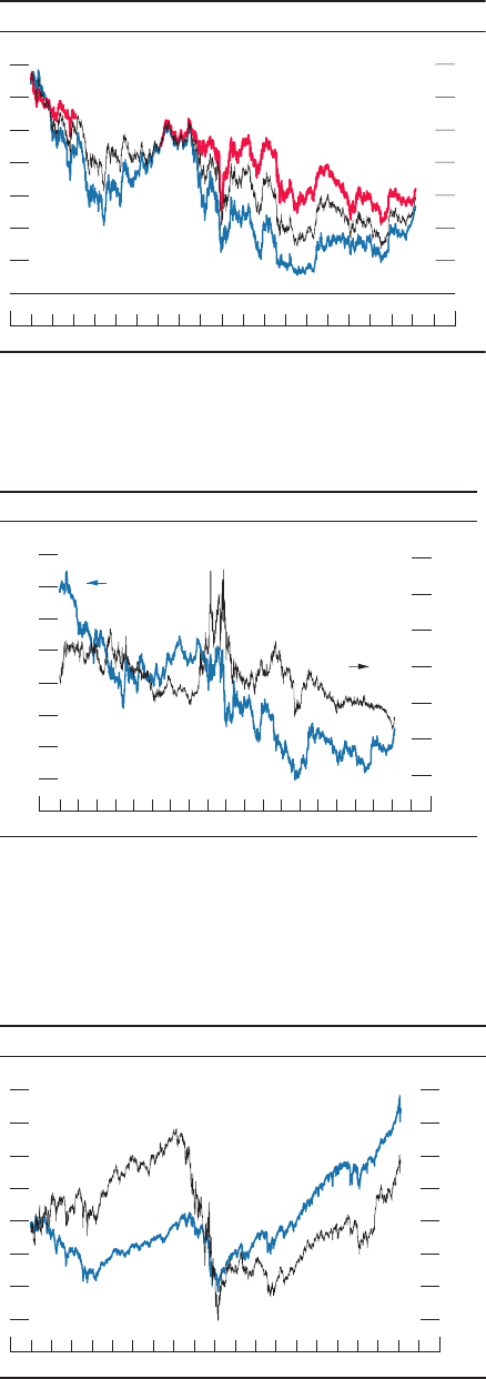
MONETARY POLICY REPORT: FEBRUARY 2018 23
increased notably in early February, ending
the period close to the median of its historical
distribution.
. . . while risk spreads on corporate bonds
have continued to decrease
Spreads on both high-yield and investment-
grade corporate bond yields over comparable-
maturity Treasury yields have decreased
further since the middle of last year, with
spreads for high-yield bonds moving closer
to the bottom of their historical ranges. The
narrowing of the spreads since the middle of
2017 appears to reect both an anticipation
that the losses from defaults on these bonds
will be smaller and a lower compensation
being charged for bearing the risk of such
losses. (For a discussion of nancial stability
issues, see the box “Developments Related to
Financial Stability.”)
Markets for Treasury securities, mortgage-
backed securities, municipal bonds, and
short-term funding have functioned well
Available indicators of Treasury market
functioning have generally remained stable
over the second half of 2017 and early 2018,
with a variety of liquidity metrics—including
bid-ask spreads, bid sizes, and estimates of
transaction costs—mostly unchanged over
the period. Liquidity conditions in the agency
MBS market have also been generally stable.
In recent months, the functioning of Treasury
and agency MBS markets has not been notably
aected by the implementation of the Federal
Reserve’s balance sheet normalization program
and the resulting reduction in reinvestment of
principal payments from the Federal Reserve’s
securities holdings. In early February, amid
nancial market volatility, liquidity conditions
in the Treasury market deteriorated but have
recovered somewhat since. Credit conditions
in municipal bond markets have also remained
generally stable since June2017. Over that
period, yield spreads on 20-year general
obligation municipal bonds over comparable-
maturity Treasury securities have narrowed
on balance. Nevertheless, signicant nancial
strains were still evident for some issuers.
S&P 500 index
25
50
75
100
125
150
175
200
December 31, 1999 = 100
2018201620142012201020082006200420022000
33. Equity prices
Daily
Dow Jones bank index
S
OURCE
: Standard & Poor's Dow Jones Indices via Bloomberg. (For
Dow
Jones Indices licensing information, see the note on the Contents page.)
Yield
0
50
100
150
200
250
300
Basis points
2
3
4
5
6
7
8
9
2018201620142012201020082006200420022000
32. Yield and spread on agency mortgage-backed securities
Percent
Spread
N
OTE: The data are daily. Yield shown is for the Fannie Mae 30-year
current coupon, the coupon rate at which new mortgage-backed securities
would be priced at par, or face, value. Spread shown is to the average of the
5- and 10-year nominal Treasury yields. The data extend through February
16, 2018.
SOURCE: Department of the Treasury; Barclays.
5-year
30-year
0
1
2
3
4
5
6
7
Percent
2018201620142012201020082006200420022000
31. Yields on nominal Treasury securities
Daily
10-year
N
OTE: The Treasury ceased publication of the 30-year constant
maturity
series on February 18, 2002, and resumed that series on February 9, 2006.
S
OURCE
: Department of the Treasury.

24 PART 1: RECENT ECONOMIC AND FINANCIAL DEVELOPMENTS
1. An overview of the framework for assessing nancial
stability in the United States is provided in Stanley Fischer
(2017), “An Assessment of Financial Stability in the United
States,” speech delivered at the IMF Workshop on Financial
Surveillance and Communication: Best Practices from
Latin America, the Caribbean, and Advanced Economies,
Washington, June27, www.federalreserve.gov/newsevents/
speech/scher20170627a.htm.
Overall vulnerabilities in the U.S. nancial system
remain moderate on balance.
1
Valuation pressures
continue to be elevated across a range of asset
classes, including equities and commercial real estate.
Vulnerabilities from leverage in the nancial sector
appear low, reecting in part capital and liquidity
ratios of banks that have continued to improve from
already strong positions. However, there are signs
that nonbank nancial leverage has been increasing
in some areas—for example, in the provision of
margin credit to equity investors such as hedge funds.
Vulnerabilities from nonnancial leverage are judged
to be moderate. While household debt balances have
been increasing modestly, the leverage of the business
sector is elevated, particularly among speculative-grade
rms. Vulnerabilities related to maturity and liquidity
transformation remain low on net.
Over the second half of 2017, valuation pressures
edged up from already elevated levels. In general,
valuations are higher than would be expected based
solely on the current level of longer-term Treasury
yields. In part reecting growing anticipation of the
boost to future (after-tax) earnings from a corporate
tax rate cut, price-to-earnings ratios for U.S. stocks
rose through January and were close to their highest
levels outside of the late 1990s (gure A); ratios
dropped back somewhat in early February. In a sign of
increasing valuation pressures in commercial real estate
markets, net operating income relative to property
values (referred to as capitalization rates) have been
declining relative to Treasury yields of comparable
maturity for multifamily and industrial properties.
While these spreads narrowed further from already
low levels, they are wider than in 2007. Even though
the aggregate residential house price-to-rent ratio has
been increasing faster than its long-run trend, it is
only slightly elevated at present. In corporate credit
markets, spreads of corporate bond yields over those
of Treasury securities with comparable maturities fell,
and the high-yield spread is now near the bottom of its
historical distribution. Spreads on leveraged loans and
collateralized loan obligations—which are a signicant
Developments Related to Financial Stability
funding source for the corporate sector—stayed
compressed. In addition, nonprice terms eased on these
types of loans, indicating weaker investor protection
than at the peak of the previous credit cycle in 2007.
Consistent with elevated risk appetite, virtual currencies
experienced sharp price increases in 2017.
Vulnerabilities related to nancial-sector leverage
appear low. Leverage at insurance companies and at
broker-dealers is on the low end of its historical range,
and most indicators of leverage at other nonbank
nancial rms are stable. However, there is some
evidence that dealers have eased price terms to hedge
funds and real estate investment trusts, and that hedge
funds have gradually increased their use of leverage,
in particular margin credit for equity trades. Although
such easing of price terms has taken place against the
backdrop of building valuation pressures, the strong
capital position of bank holding companies reduces
the risk that sudden drops in asset prices could
signicantly affect bank-afliated dealers. Risk-based
regulatory capital ratios for most of the largest bank
holding companies continued to increase from already
high levels.
If interest rates were to increase unexpectedly,
banks’ strong capital position should help absorb the
consequent losses on securities. About one-third of
the losses that could be experienced by banks would
affect held-to-maturity securities. While these losses
5
10
15
20
25
30
Ratio
201820142010200620021998199419901986
A. Forward price-to-earnings ratio of S&P 500 firms
Monthly
Historical median
N
OTE: The February 2018 value is based on a mid-month estimate.
The
data
depict the aggregate forward price-to-earnings ratio of S&P 500
firms.
The
historical median is based on data from 1985 to the present. Shaded
bars
indicate
periods of recession as defined by the National Bureau of
Economic
Research. Data are based on 12-month-ahead expected earnings per share.
S
OURCE
: Staff estimates based on Thomson Reuters, IBES.
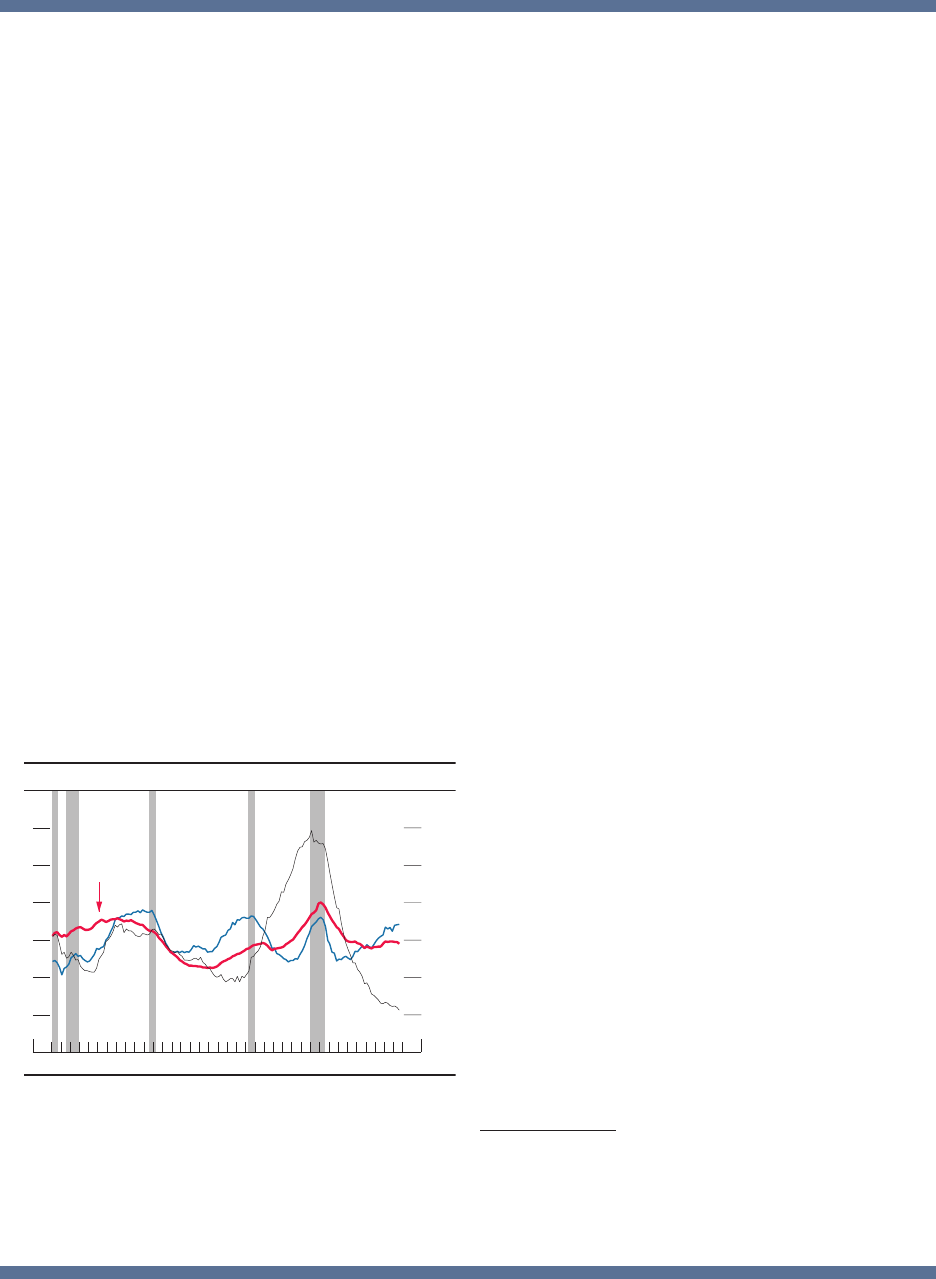
MONETARY POLICY REPORT: FEBRUARY 2018 25
would not reduce regulatory capital, they could still
have a variety of negative consequences—for example,
by worsening banks’ funding terms. The large share of
deposits in bank liabilities is also likely to soften the
effect of an unexpected rise in interest rates on banks,
because deposit rates tend to adjust with a delay and
bank protability would improve in the meantime.
Overall vulnerabilities arising from leverage in
the nonnancial sector continue to be moderate.
Continuing its pattern in recent years, household debt
has expanded about in line with nominal income,
and the household credit-to-GDP gap remains sizable
and negative (gure B). Leverage in the nonnancial
business sector remains high, with net issuance of risky
debt climbing in recent months. However, the share of
the lowest-quality debt in total issuance declined, and
relatively low interest expenses mitigated some of the
vulnerabilities associated with elevated leverage.
In part attributable to regulations introduced
since the nancial crisis, vulnerabilities associated
with liquidity and maturity transformation—that is,
the nancing of illiquid or long-maturity assets with
short-maturity debt—continue to be low. The reliance
of global systemically important banks (G-SIBs) on
short-term wholesale funding has risen only slightly
from post-crisis lows, while their holdings of high-
quality liquid assets stand at high levels and exceed
those required by the Liquidity Coverage Ratio. The
share of core deposits in total liabilities at G-SIBs
also remains at historically high levels. More than
one year after the money market fund reform, which
reduced run risk as investors shifted from prime to
government funds, the growth in alternative short-
term investment vehicles has been limited. Regarding
securitized products, although the issuance of asset-
backed securities (ABS) was strong, overall issuance
has remained well below pre-crisis levels for most asset
classes, and securitizations appear to involve limited
maturity or liquidity transformation. Nonetheless, ABS
issuance was boosted by the securitization of assets
that were rarely securitized in the past, such as aircraft
leases and mobile phone contracts. In addition, certain
nontraditional liabilities of life insurers, including
funding-agreement-backed securities, have grown
notably recently, although levels remain low relative to
the broader market for securitizations.
Financial vulnerabilities in foreign economies are
moderate overall. Advanced foreign economies, many
of which have strong nancial and real linkages to
the United States, continue to struggle with elevated
valuations, the disposal of legacy assets, and, in some
cases, worrisome rises in mortgage debt. Some major
emerging market economies harbor more pronounced
vulnerabilities, reecting one or more of the following:
substantial corporate leverage, scal concerns, or
excessive reliance on foreign funding.
The countercyclical capital buffer (CCyB) is a
macroprudential tool the Federal Reserve Board can
use to increase the resilience of the nancial system
by raising capital requirements on internationally
active banking organizations. The CCyB is activated
when there is an elevated risk of above-normal future
losses and when the banking organizations for which
capital requirements would be raised by the buffer
are exposed to or are contributing to this elevated
risk—either directly or indirectly. The nancial stability
developments, assessments, and framework described
and used here bear importantly on the Board’s setting
of the CCyB.
2
In December2017, the Board voted to
afrm the CCyB at its level of 0percent.
2. See Board of Governors of the Federal Reserve System
(2016), “Regulatory Capital Rules: The Federal Reserve Board’s
Framework for Implementing the U.S. Basel III Countercyclical
Capital Buffer,” nal policy statement (Docket No. R-1529),
Federal Register, vol. 81 (September16), pp. 63682–88.
Corporate business
Noncorporate business
10
5
+
_
0
5
10
15
Percentage point difference from trend
2017201320092005200119971993198919851981
Quarterly
B. Private nonfinancial sector credit-to-GDP gap
NOTE: The data extend through 2017:Q3 and are smoothed using
a
Hodrick-Prescott
filter. The shaded bars indicate periods of
business
recession
as defined by the National Bureau of Economic Research.
Gaps
have
been weighted by their share of overall credit. GDP is gross
domestic
product.
SOURCE
: Federal Reserve Board, Statistical Release Z.1,
“Financial
Accounts
of the United States”; Bureau of Economic Analysis via
Haver
Analytics,
national income and product accounts, Table 1.1.5:
Gross
Domestic Product; Board staff calculations.
Household
(continued on next page)

26 PART 1: RECENT ECONOMIC AND FINANCIAL DEVELOPMENTS
Over the second half of 2017, the Federal Reserve
Board has taken some key steps to reduce regulatory
burden while promoting the nancial stability of the
United States. The Federal Reserve Board, Ofce of
the Comptroller of the Currency, and Federal Deposit
Insurance Corporation jointly proposed amendments
to the banking agencies’ commercial real estate
appraisal regulations that raised the threshold price
for mandating appraisals from $250,000 to $400,000,
thereby reducing the number of required appraisals.
3
In addition, the federal banking agencies issued a
proposal to simplify aspects of community banking
organizations’ regulatory capital rules, with the goal
of reducing regulatory burden on smaller institutions
while maintaining the safety and soundness of the
banking system.
4
The Board requested comment on a corporate
governance proposal to enhance the effectiveness
of nancial rms’ boards of directors. The proposal
refocuses the Federal Reserve’s supervisory expectations
for the largest rms’ boards of directors on their core
responsibilities and would also reduce unnecessary
burden for the boards of smaller institutions.
5
The Board
3. See Ofce of the Comptroller of the Currency, Board
of Governors of the Federal Reserve System, and the
Federal Deposit Insurance Corporation (2017), “Real Estate
Appraisals,” notice of proposed rulemaking and request for
comment (Docket No. R-1568), Federal Register, vol. 82
(July31), pp. 35478–93.
4. See Ofce of the Comptroller of the Currency, Board
of Governors of the Federal Reserve System, and the Federal
Deposit Insurance Corporation (2017), “Simplications to the
Capital Rule Pursuant to the Economic Growth and Regulatory
Paperwork Reduction Act of 1996,” notice of proposed
rulemaking (Docket No. R-1576), Federal Register, vol. 82
(October27), pp. 49984–50044.
5. See Board of Governors of the Federal Reserve System
(2017), “Federal Reserve Board Invites Public Comment on
also adopted a nal rule to improve the resolvability
and resilience of G-SIBs and their subsidiaries to
restrictions regarding the terms of their noncleared
qualied nancial contracts.
6
In addition, the Board
proposed changes to its supervisory rating system
for large nancial institutions to better align with the
post-crisis supervisory program for these rms; smaller
institutions, including community banks, would
continue to use the current rating system.
7
Finally, the
Board requested comment on a package of proposals
that would increase the transparency of its stress-testing
program. In particular, the proposals would provide
more information about the models used to estimate
hypothetical losses in the stress tests while maintaining
the Board’s ability to test the resilience of the nation’s
largest and most complex banks.
8
Two Proposals; Corporate Governance and Rating System
for Large Financial Institutions,” press release, August3,
https://www.federalreserve.gov/newsevents/pressreleases/
bcreg20170803a.htm.
6. See Board of Governors of the Federal Reserve System
(2017), “Restrictions on Qualied Financial Contracts of
Systemically Important U.S. Banking Organizations and the
U.S. Operations of Systemically Important Foreign Banking
Organizations; Revisions to the Denition of Qualifying
Master Netting Agreement and Related Denitions,” nal rule
(Docket No. R-1538), Federal Register, vol. 82 (September12),
pp. 42882–926.
7. See Board of Governors, “Federal Reserve Board Invites
Public Comment on Two Proposals,” in note 5.
8. See Board of Governors of the Federal Reserve System
(2017), “Federal Reserve Board Requests Comment on
Package of Proposals That Would Increase the Transparency
of Its Stress Testing Program,” press release, December7,
www.federalreserve.gov/newsevents/pressreleases/
bcreg20171207a.htm.
Developments Related to Financial Stability (continued)
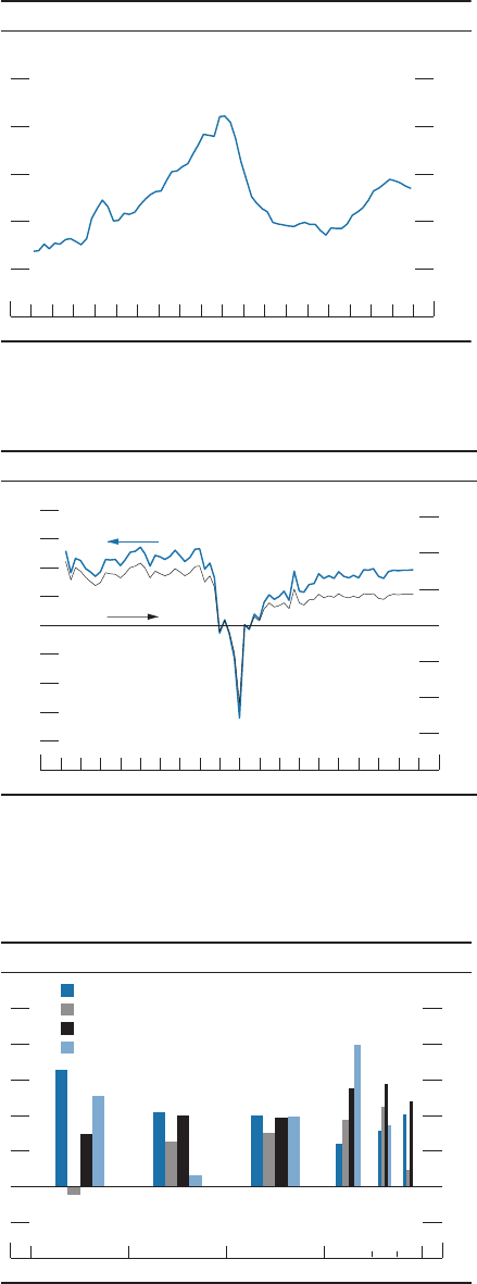
MONETARY POLICY REPORT: FEBRUARY 2018 27
In particular, prices for Puerto Rico general
obligation bonds fell notably after Hurricane
Maria hit the island and its economic outlook
deteriorated even further. However, these
developments left little imprint in broader
municipal bond markets. Conditions in
domestic short-term funding markets have
remained stable since the middle of last year.
Bank credit continued to expand and
bank protability remained stable
Aggregate credit provided by commercial
banks continued to expand in the second
half of 2017 at a pace similar to the one seen
earlier in the year but more slowly than in
2016. Its pace was also slower than that of
nominal GDP, thus leaving the ratio of total
commercial bank credit to current-dollar GDP
slightly lower than earlier in 2017 (gure34).
Measures of bank protability were little
changed at levels below their historical
averages (gure35).
International Developments
Economic activity in most foreign
economies continued at a healthy pace in
the second half of 2017
Foreign real GDP appears to have expanded
notably in the second half of 2017, extending
the period since mid-2016 when the pace of
economic growth picked up broadly around
the world.
Growth in advanced foreign economies
was solid, and unemployment fell to
multidecade lows . . .
In the advanced foreign economies (AFEs),
the economic recovery has continued to rm.
Real GDP in the euro area and the United
Kingdom expanded at a solid pace in the
second half of the year (gure36). Economic
activity also continued to expand in Japan,
though real GDP growth slowed sharply in
the fourth quarter. In Canada, data through
November indicate that economic growth
moderated somewhat in the second half
following a very rapid expansion earlier in
the year. Unemployment declined further as
1
+
_
0
1
2
3
4
5
Percent, annual rate
2017201620152014
36. Real gross domestic product growth in selected
advanced foreign economies
H1
Q3
Q4
N
OTE:The data for the United Kingdom and the euro area
incorporate
flash estimates for 2017:Q4. The data for Japan incorporate the
preliminary
estimate for 2017:Q4. The data for Canada extend through 2017:Q3.
S
OURCE
:
For the United Kingdom, Office for National Statistics; for Japan,
Cabinet Office, Government of Japan; for the euro area, Eurostat; for
Canada,
Statistics Canada; all via Haver Analytics.
United Kingdom
Japan
Euro area
Canada
Return on assets
30
20
10
+
_
0
10
20
30
Percent, annual rate
2.0
1.5
1.0
.5
+
_
0
.5
1.0
1.5
2.0
201720152013201120092007200520032001
35. Profitability of bank holding companies
Percent, annual rate
Return on equity
N
OTE: The data are quarterly and are seasonally adjusted. The data
extend
through 2017:Q3.
SOURCE: Federal Reserve Board, Form FR Y-9C, Consolidated
Financial
Statements for Bank Holding Companies.
55
60
65
70
75
Percent
201720152013201120092007200520032001
34. Ratio of total commercial bank credit to nominal gross
domestic product
Quarterly
SOURCE
: Federal Reserve Board, Statistical Release H.8, “Assets
and
Liabilities
of Commercial Banks in the United States”; Bureau of
Economic
Analysis via Haver Analytics.

28 PART 1: RECENT ECONOMIC AND FINANCIAL DEVELOPMENTS
well, reaching 40-year lows in Canada and
the United Kingdom, while growth in labor
compensation ticked up only modestly.
. . . but ination remained subdued . . .
Consumer price ination rose somewhat in
most AFEs, boosted by the rise in commodity
prices (gure37). However, headline and
especially core ination remained below the
central banks’ targets in the euro area and
Japan. In contrast, U.K. ination rose further
above the Bank of England’s (BOE) 2percent
target as the substantial sterling depreciation
observed since the June2016 Brexit
referendum continued to provide some uplift
to import prices. (For more discussion
of ination both in the United States and
abroad, see the box “Low Ination in the
Advanced Economies” in the Domestic
Developments section.)
. . . leading AFE central banks to maintain
accommodative monetary policies
The Bank of Japan kept its policy rates at
historically low levels, with the target for
10-year government bond yields around
zero. In October, the European Central Bank
extended its asset purchase program until
September2018, albeit at a reduced pace. The
Bank of Canada and the BOE both raised
their policy rates but also indicated that they
intend to proceed gradually with further
removal of policy accommodation.
In emerging Asia, growth remained solid. . .
Economic growth in China remained relatively
strong in the second half of 2017 even as the
authorities enacted policies to limit production
in heavily polluting industries, tighten nancial
regulations, and curb house price growth
(gure38). Most other emerging Asian
economies registered very strong growth in the
third quarter of 2017, fueled by solid external
demand, but slowed in the fourth quarter.
United Kingdom
Canada
Euro area
1
+
_
0
1
2
3
4
12-month percent change
2014 2015 2016 2017 2018
37. Consumer price inflation in selected advanced foreign
economies
Monthly
Japan
N
OTE
:
The data for the euro area incorporate the flash estimate for January
2018. The data for Canada and Japan extend through December 2017.
SOURCE:
For the United Kingdom, Office for National Statistics; for Japan,
Ministry of International Affairs and Communications; for the euro
area,
Statistical Office of the European Communities; for Canada,
Statistics
Canada; all via Haver Analytics.
6
3
+
_
0
3
6
9
12
Percent, annual rate
2017201620152014
38. Real gross domestic product growth in selected
emerging market economies
H1
Q3
Q4
N
OTE: The data for China are seasonally adjusted by Board staff. The
data
for
Korea, Mexico, and Brazil are seasonally adjusted by their
respective
government
agencies. The data for Mexico incorporate the flash estimate
for
2017:Q4. The data for Brazil extend through 2017:Q3.
SOURCE: For China, China National Bureau of Statistics; for Korea,
Bank
of
Korea; for Mexico, Instituto Nacional de Estadistica y Geografia;
for
Brazil, Instituto Brasileiro de Geografia e Estatistica; all via Haver Analytics.
China
Korea
Mexico
Brazil
MONETARY POLICY REPORT: FEBRUARY 2018 29
. . . while the largest Latin American
economies continued to struggle
In Mexico, real GDP declined in the third
quarter as two major earthquakes and a
hurricane signicantly disrupted economic
activity, but rebounded in the fourth quarter.
Following a prolonged period of contraction,
the Brazilian economy continues to recover,
but only at a weak pace. Private investment has
remained sluggish amid corporate deleveraging
and continued uncertainty about government
policies, although it turned positive in the third
quarter for the rst time in nearly four years.
Foreign equity prices rose further on net. . .
Solid macroeconomic data and robust
corporate earnings helped broad AFE and
emerging market economies (EMEs) equity
indexes extend their 2016 gains through the
start of this year (gure39). Declines since
the end of January have erased some of these
gains, and volatility in foreign stock markets
increased. On balance, most AFE stock
prices are higher, and EME equity markets
signicantly outperformed those of AFEs.
Capital ows into emerging market mutual
funds generally remained robust as higher
commodity prices added to optimism about
the economic outlook (gure40).
. . . and government bond yields
increased
Longer-term government bond yields in most
AFEs were noticeably higher than their mid-
2017 levels, reecting strengthening growth
and mounting prospects for the normalization
of monetary policies (gure41). In Canada,
where the central bank has raised its policy
interest rate 75 basis points since June, the rise
in longer-term yields was particularly notable.
On balance, spreads of dollar-denominated
emerging market sovereign bonds over U.S.
Treasury securities were stable around the
levels observed in mid-2017 (as shown in
gure40).
EMBI+ (left axis)
60
40
20
+
_
0
20
40
60
Billions of dollars
250
300
350
400
450
500
2014 2015 2016 2017 2018
40. Emerging market mutual fund flows and spreads
Basis points
Jan.
Feb.
N
OTE
: The bond and equity fund flow data are quarterly sums of
weekly
data from January 1, 2014, to December 31, 2017, and monthly sums
of
weekly data from January 1, 2018, to February 14, 2018. The fund flows data
exclude funds located in China. The J.P. Morgan Emerging Markets
Bond
Index Plus (EMBI+) data are weekly averages of daily data and
extend
through February 20, 2018.
S
OURCE
: For bond and equity fund flows, EPFR Global; for EMBI+,
J.P.
Morgan Emerging Markets Bond Index Plus via Bloomberg.
Bond fund flows (right axis)
Equity fund flows (right axis)
United Kingdom
Emerging market economies
Euro area
85
90
95
100
105
110
115
120
125
130
135
140
145
150
Week ending January 8, 2014 = 100
2014 2015 2016 2017 2018
39. Equity indexes for selected foreign economies
Weekly
Japan
N
OTE
: The data are weekly averages of daily data and extend
through
February 21, 2018.
S
OURCE: For euro area, DJ Euro Stoxx Index; for Japan, TOPIX
Stock
Index; for United Kingdom, FTSE 100 Stock Index; for emerging
market
economies, MSCI Emerging Markets Local Currency Index; all
via
Bloomberg.
30 PART 1: RECENT ECONOMIC AND FINANCIAL DEVELOPMENTS
The dollar depreciated on net
The broad dollar index––a measure of the
trade-weighted value of the dollar against
foreign currencies––fell roughly 5percent in
the rst half of 2017. Notwithstanding some
appreciation in early February, the currency
has depreciated further since the end of June,
partially reversing substantial appreciation
realized over the period from 2014 to 2016
(gure42). The weakness in the dollar mostly
reects a broad-based improvement in the
outlook for foreign economic growth. Brexit-
related headlines weighed on the British pound
at times during the second half of 2017, but
progress regarding the terms of the U.K.
separation from the European Union boosted
the currency later in the year. In contrast,
the dollar appreciated against the Mexican
peso, on net, amid uncertainty around North
American Free Trade Agreement negotiations.
Canada
United States
Germany
.5
+
_
0
.5
1.0
1.5
2.0
2.5
3.0
Percent
2014 2015 2016 2017 2018
41. Nominal 10-year government bond yields in
selected advanced economies
Weekly
United Kingdom
N
OTE
: The data are weekly averages of daily benchmark yields and
extend
through February 21, 2018.
S
OURCE
:Bloomberg.
Mexican peso
British pound
Euro
90
100
110
120
130
140
150
160
170
Week ending January 8, 2014 = 100
2014 2015 2016 2017 2018
42. U.S. dollar exchange rate indexes
Weekly
Broad dollar
Dollar appreciation
N
OTE: The data, which are in foreign currency units per dollar, are
weekly
averages of daily data and extend through February 21, 2018. As indicated by
the
arrow, increases in the data represent U.S. dollar appreciation,
and
decreases represent U.S. dollar depreciation.
SOURCE: Federal Reserve Board, Statistical Release H.10,
“Foreign
Exchange Rates.”
31
The Federal Open Market Committee
raised the federal funds rate target range
in December
For more than two years, the Federal Open
Market Committee (FOMC) has been
gradually increasing its target range for
the federal funds rate as the labor market
strengthened and headwinds in the aftermath
of the recession continued to abate. After
having raised the target range for the federal
funds rate twice in the rst half of 2017,
the Committee raised it again in December,
bringing the target range to 1¼ to 1½percent
(gure43).
10
As on previous occasions, the
decision to increase the federal funds rate in
December reected realized and expected labor
market conditions and ination relative to the
FOMC’s objectives. Information available at
that time indicated that economic activity had
been rising at a solid rate and the labor market
had continued to strengthen. In addition,
although ination had continued to run below
the FOMC’s 2percent longer-run objective,
10. See Board of Governors of the Federal Reserve
System (2017), “Federal Reserve Issues FOMC
Statement,” press release, December13, https://
www.federalreserve.gov/newsevents/pressreleases/
monetary20171213a.htm.
the Committee expected that it would stabilize
around that target over the medium term. At
its most recent meeting, which concluded on
January31, the Committee kept the target
range for the federal funds rate unchanged.
11
Monetary policy continues to support
economic growth
Even with the gradual increases in the federal
funds rate to date, the Committee judges
that the stance of monetary policy remains
accommodative, thereby supporting strong
labor market conditions and a sustained return
to 2percent ination. The federal funds rate
remains somewhat below most estimates of its
neutral rate—that is, the level of the federal
funds rate that is neither expansionary nor
contractionary.
In evaluating the stance of monetary policy,
policymakers routinely consult prescriptions
from a variety of policy rules, which can
serve as useful benchmarks. However, the
11. See Board of Governors of the Federal
Reserve System (2018), “Federal Reserve Issues
FOMC Statement,” press release, January31, https://
www.federalreserve.gov/newsevents/pressreleases/
monetary20180131a.htm.
Target range for the federal funds rate
2-year Treasury rate
0
1
2
3
4
5
Percent
2008 2009 2010 2011 2012 2013 2014 2015 2016 2017 2018
43. Selected interest rates
Daily
10-year Treasury rate
N
OTE
: The 2-year and 10-year Treasury rates are the constant-maturity yields based on the most actively traded securities.
S
OURCE
: Department of the Treasury; Federal Reserve Board.
Part 2
monetary PoLicy

32 PART 2: MONETARY POLICY
use and interpretation of such prescriptions
require careful judgments about the choice
and measurement of the inputs to these
rules as well as the implications of the many
considerations these rules do not take into
account (see the box “Monetary Policy Rules
and Their Role in the Federal Reserve’s Policy
Process”).
Future changes in the federal funds rate
will depend on the economic outlook as
informed by incoming data
The Committee has continued to emphasize
that, in determining the timing and size of
future adjustments to the target range for
the federal funds rate, it will assess realized
and expected economic conditions relative to
its objectives of maximum employment and
2percent ination. This assessment will take
into account a wide range of information,
including measures of labor market
conditions, indicators of ination pressures
and ination expectations, and readings on
nancial and international developments.
The FOMC has emphasized that it will
carefully monitor actual and expected ination
developments relative to its symmetric ination
goal, as ination has been running persistently
below the 2percent longer-run objective.
The Committee expects that the ongoing
strength in the economy will warrant further
gradual increases in the federal funds rate,
and that the federal funds rate will likely
remain, for some time, below the levels that
the Committee expects to prevail in the
longer run. Consistent with this outlook,
in the most recent Summary of Economic
Projections, which was compiled at the time of
the December FOMC meeting, the median of
participants’ assessments for the appropriate
level of the midpoint of the target range
for the federal funds rate at year-end rises
gradually over the period from 2018 to 2020,
remaining below the median projection for its
longer-run level through the end of 2019.
12
12. See the December Summary of Economic
Projections, which appeared as an addendum to the
The size of the Federal Reserve’s balance
sheet has begun to decrease
The Committee had communicated for some
time that it intended to reduce the size of
the Federal Reserve’s balance sheet once
normalization of the level of the federal funds
rate was well under way. At its meeting in
September, the FOMC decided to initiate the
balance sheet normalization program described
in the June2017 Addendum to the Policy
Normalization Principles and Plans. This
program is gradually and predictably reducing
the Federal Reserve’s securities holdings by
decreasing the reinvestment of the principal
payments it receives from securities held in the
System Open Market Account (SOMA). Since
October, such payments have been reinvested
only to the extent that they exceeded gradually
rising caps (gure44).
In the fourth quarter, the Open Market Desk
at the Federal Reserve Bank of New York, as
directed by the Committee, reinvested principal
payments from the Federal Reserve’s holdings
of Treasury securities maturing during each
calendar month in excess of $6billion. The
Desk also reinvested in agency mortgage-
backed securities (MBS) the amount of
principal payments from the Federal Reserve’s
holdings of agency debt and agency MBS
received during each calendar month in excess
of $4billion. Since January, payments of
principal from maturing Treasury securities
and from the Federal Reserve’s holdings
of agency debt and agency MBS have been
reinvested to the extent that they have exceeded
$12billion and $8billion, respectively. The
Committee has indicated that the cap for
Treasury securities will continue to increase
in steps of $6billion at three-month intervals
until it reaches $30billion per month, and
that the cap for agency debt and agency MBS
will continue to increase in steps of $4billion
at three-month intervals until it reaches
$20billion per month. These caps will remain
in place until the Committee judges that the
Federal Reserve is holding no more securities
minutes of the December12–13, 2017, meeting of the
FOMC and is presented in Part 3 of this report.
MONETARY POLICY REPORT: FEBRUARY 2018 33
than necessary to implement monetary policy
eciently and eectively.
The initiation of the balance sheet
normalization program was widely anticipated
and therefore did not elicit a notable reaction
in nancial markets. Subsequently, the
implementation of the program has proceeded
smoothly without materially aecting Treasury
and MBS markets. With the caps having
been set thus far at relatively low levels, the
reduction in SOMA securities has represented
a small fraction of the SOMA securities
holdings. Consequently, the Federal Reserve’s
total assets have declined somewhat to about
$4.4 trillion, with holdings of Treasury
securities at approximately $2.4 trillion and
holdings of agency debt and agency MBS at
approximately $1.8 trillion (gure45).
Interest income on the SOMA portfolio has
continued to support substantial remittances
to the U.S. Treasury. Preliminary nancial
statement results indicate that the Federal
Billions of dollars
Treasury securities
Monthly Billions of dollars
Agency debt and mortgage-backed securities
Monthly
N
: Reinvestment and redemption amounts of agency mortgage-backed securities are projections starting in January 2018. The
data extend through December 2019.
S: Federal Reserve Bank of New York; Federal Reserve Board sta calculations.
44. Principal payments on SOMA securities
10
20
30
40
50
60
70
80
201920182017
Monthly cap
Redemptions
Reinvestments
10
20
30
40
50
60
70
80
201920182017
Monthly cap
Redemptions
Reinvestments
Trillions of dollars
2008 2009 2010 2011 2012 2013 2014 2015 2016 2017 2018
45. Federal Reserve assets and liabilities
Weekly
Assets
Liabilities and capital
Other assets
Credit and liquidity
facilities
Agency debt and mortgage-backed securities holdings
Treasury securities held outright
Federal Reserve notes in circulation
Deposits of depository institutions
Capital and other liabilities
5.0
4.5
4.0
3.5
3.0
2.5
2.0
1.5
1.0
.5
0
.5
1.0
1.5
2.0
2.5
3.0
3.5
4.0
4.5
5.0
N
OTE
: “Credit and liquidity facilities” consists of primary, secondary, and seasonal credit; term auction credit; central bank liquidity swaps; support for
Maiden
Lane, Bear Stearns, and AIG; and other credit facilities, including the Primary Dealer Credit Facility, the Asset-Backed Commercial Paper Money
Market
Mutual Fund Liquidity Facility, the Commercial Paper Funding Facility, and the Term Asset-Backed Securities Loan Facility. “Other assets” includes
unamortized
premiums and discounts on securities held outright. “Capital and other liabilities” includes reverse repurchase agreements, the U.S. Treasury
General Account, and the U.S. Treasury Supplementary Financing Account. The data extend through February 14, 2018.
S
OURCE
: Federal Reserve Board, Statistical Release H.4.1, “Factors Affecting Reserve Balances.”
34 PART 2: MONETARY POLICY
Reserve remitted about $80.2 billion of its
estimated 2017 net income to the Treasury.
The Federal Reserve’s implementation of
monetary policy has continued smoothly
In December2017, the Federal Reserve raised
the eective federal funds rate by increasing
the interest rate paid on reserve balances along
with the interest rate oered on overnight
reverse repurchase agreements (ON RRPs).
Specically, the Federal Reserve increased
the interest rate paid on required and excess
reserve balances to 1½percent and the ON
RRP oering rate to 1¼percent. In addition,
the Board of Governors approved an increase
in the discount rate (the so-called primary
credit rate) to 2percent. Yields on a broad set
of money market instruments moved higher
in response to the FOMC’s policy action in
December. The eective federal funds rate rose
in line with the increase in the FOMC’s target
range and generally traded near the middle
of the new target range amid orderly trading
conditions in money markets. Usage of the
ON RRP facility has declined on net since the
middle of 2017, reecting relatively attractive
yields on alternative investments.
Although the normalization of the monetary
policy stance has proceeded smoothly, the
Federal Reserve has continued to test the
operational readiness of other policy tools as
part of prudent planning. Two operations of
the Term Deposit Facility were conducted in
the second half of 2017; seven-day deposits
were oered at both operations with a oating
rate of 1 basis point over the interest rate
on excess reserves. In addition, the Desk
conducted several small-value exercises solely
for the purpose of maintaining operational
readiness.

MONETARY POLICY REPORT: FEBRUARY 2018 35
the three key principles of good monetary policy
noted earlier. Each rule takes into account estimates
of how far away the economy is from achieving the
Federal Reserve’s dual-mandate goals of maximum
employment and price stability. Specically, most of
the rules include the difference between the rate of
unemployment that is sustainable in the longer run (u
LR
)
and the current unemployment rate (the unemployment
gap); the rst-difference rule includes the change in the
unemployment gap rather than its level.
3
In addition,
most of the rules include the difference between
ination and its longer-run objective (2percent as
measured by the annual change in the price index
for personal consumption expenditures (PCE), in the
case of the Federal Reserve), while the price-level rule
includes the gap between the level of prices today
and the level of prices that would be observed if
ination had been constant at 2percent from a
specied starting year.
The Taylor (1993), balanced-approach, adjusted
Taylor (1993), and price-level rules provide
prescriptions for the level of the federal funds rate and
require an estimate of the neutral real interest rate in
the longer run (r
LR
)—that is, the level of the real federal
What are monetary policy rules?
Monetary policy rules are formulas that prescribe
the setting of a policy rate, such as the federal funds
rate, that should prevail in relation to the values of a
small number of other variables—typically including
the gap between actual and target ination along with
an estimate of resource slack in the economy. Policy
rules can provide helpful guidance for policymakers.
Indeed, since 2004, prescriptions from policy rules
have been part of the information regularly reported
to the Federal Open Market Committee (FOMC)
ahead of its meetings.
1
However, interpretation of the
prescriptions of policy rules requires careful judgment
about the measurement of the inputs to the rules and
the implications of the many considerations the rules
do not take into account.
Policy rules can incorporate key principles of good
monetary policy. One key principle is that monetary
policy should respond in a predictable way to changes
in economic conditions. A second key principle is
that monetary policy should be accommodative when
ination is below the desired level and employment
is below its maximum sustainable level; conversely,
monetary policy should be restrictive when the
opposite holds. A third key principle is that, to stabilize
ination, the policy rate should be adjusted by more
than one-for-one in response to persistent increases or
decreases in ination.
Economists have analyzed many monetary policy
rules, including the well-known Taylor (1993) rule
as well as other rules that will be discussed later: the
“balanced approach” rule, the “adjusted Taylor (1993)”
rule, the “price level” rule, and the “rst difference”
rule (gure A).
2
These policy rules generally embody
Monetary Policy Rules and Their Role in the Federal Reserve’s
Policy Process
1. Prescriptions from monetary policy rules are included
in the Board staff’s Tealbook (previously the Bluebook); the
precise set of rules presented has changed from time to time.
The transcripts and brieng materials for FOMC meetings
through 2012 are available on the Board’s website at https://
www.federalreserve.gov/monetarypolicy/fomc_historical.
htm. In the materials from 2012, the policy rule prescriptions
are contained in the Monetary Policy Strategies section of
Tealbook B. The brieng materials that FOMC policymakers
review regularly also include the Board staff’s baseline
forecast for the economy and model simulations of a variety of
alternative scenarios intended to provide a sense of the effects
of other plausible developments that were not included in the
staff’s baseline forecast.
2. The Taylor (1993) rule was rst suggested in John B.
Taylor (1993), “Discretion versus Policy Rules in Practice,”
Carnegie-Rochester Conference Series on Public Policy, vol.39
(December), pp. 195–214. The balanced-approach rule was
analyzed in John B. Taylor (1999), “A Historical Analysis of
Monetary Policy Rules,” in John B. Taylor, ed., Monetary Policy
Rules (Chicago: University of Chicago Press), pp.319–41. The
adjusted Taylor (1993) rule was studied in David Reifschneider
and John C. Williams (2000), “Three Lessons for Monetary
Policy in a Low-Ination Era,” Journal of Money, Credit, and
Banking, vol. 32 (November), pp. 936–66. A price-level rule
was discussed in Robert E. Hall (1984), “Monetary Strategy
with an Elastic Price Standard,” in Price Stability and Public
Policy, proceedings of a symposium sponsored by the Federal
Reserve Bank of Kansas City, held in Jackson Hole, Wyo.,
August2–3 (Kansas City: Federal Reserve Bank of Kansas
City), pp. 137–59, https://www.kansascityfed.org/publicat/
sympos/1984/s84.pdf. Finally, the rst-difference rule was
introduced by Athanasios Orphanides (2003), “Historical
Monetary Policy Analysis and the Taylor Rule,” Journal
of Monetary Economics, vol. 50 (July), pp. 983–1022. A
comprehensive review of policy rules is in John B. Taylor
and John C. Williams (2011), “Simple and Robust Rules for
Monetary Policy,” in Benjamin M. Friedman and Michael
Woodford, eds., Handbook of Monetary Economics, vol.3B
(Amsterdam: North-Holland), pp. 829–59. The same volume
of the Handbook of Monetary Economics also discusses
approaches other than policy rules for deriving policy rate
prescriptions.
3. The Taylor (1993) rule represented slack in resource
utilization using an output gap (the difference between the
current level of real gross domestic product (GDP) and what
GDP would be if the economy was operating at maximum
employment). The rules in gure A represent slack in resource
utilization using the unemployment gap instead, because that
gap better captures the FOMC’s statutory goal to promote
maximum employment. Movements in these alternative
(continued on next page)
36 PART 2: MONETARY POLICY
In four of the rules, the interest rate responds to
deviations of ination from its longer-run value of
2percent; in the price-level rule, however, the interest
rate responds to the price-level gap (PLgap
t
). This
gap measures how far the price level is from where it
would have been had it been increasing at 2percent
each year.
5
The price-level rule thereby takes account
of deviations of ination from the longer-run objective
in earlier periods as well in the current period. Thus,
if ination has been running persistently above the
central bank’s objective, the price-level rule would
prescribe a higher policy interest rate than rules that use
the current ination gap. Likewise, if ination has been
running persistently below the central bank’s objective,
a price-level rule would prescribe setting the policy
rate lower than rules that use the current ination gap.
The purpose of this dependence on previous ination
funds rate that is expected to be consistent in the longer
run with sustained maximum employment and stable
ination.
4
In contrast, the rst-difference rule prescribes
how the level of the federal funds rate at a given time
should be altered from its previous level—that is, it
indicates how the existing rate should be increased or
decreased in a particular period.
The adjusted Taylor (1993) rule recognizes that
the federal funds rate cannot be reduced materially
below zero, and that following the prescriptions of
the Taylor (1993) rule after a period when interest
rates have been constrained may not provide enough
policy accommodation. To make up for the cumulative
shortfall in accommodation (Z
t
), the adjusted rule
prescribes only a gradual return of the policy rate to
the (positive) levels prescribed by the unadjusted Taylor
(1993) rule as the economy recovers.
measures of resource utilization are highly correlated. For
more information, see the note below gure A.
4. Taylor-type rules—including John Taylor’s original
rule—have often been estimated assuming that the value of
the neutral real interest rate in the longer run, r
LR
, is equal to
2percent, which roughly corresponds to the average historical
value of the real federal funds rate before the nancial crisis.
5. Estimation of the price-level rule requires selecting a
starting year for the price level from which to cumulate the
2percent annual ination. For the U.S. economy, 1998 is used
as the starting year; around that time, the underlying trend
of ination and longer-term ination expectations stabilized
at a level consistent with PCE price ination being close to
2percent.
NOTE:
Taylor (1993) rule
93
= + + 0.5
(
−
)
+(
− )
= + + 0.5
(
−
)
+2(
− )
Taylor (1993) rule, adjusted
93
= {
93
− ,0}
= { + +
(
−
)
+0.5
( )
,0}
=
−1
+ 0.5
(
−
)
+
(
−
)
−(
−4
−
−4
)
A. Monetary policy rules
Balanced-approach rule
Price-level rule
First-difference rule
93
, ,
93
, , and represent the values of the nominal federal funds rate prescribed by
the Taylor (1993), balanced-approach, adjusted Taylor (1993), price-level, and rst
-dierence rules, respectively.
denotes the actual nominal federal funds rate for quarter t, is four-quarter price ination for quarter t,
is the unemployment rate in quarter t,and is the level of the neutral real federal funds rate in the longer
run that, on average, is expected to be consistent with sustaining maximum employment and ination at its
2p
ercent longer-run objective,
. In addition, is the rate of unemployment in the longer run. is the
cumulative su
m of past deviations of the federal funds rate from the prescriptions of the Taylor (1993) rule when
that rule prescribes setting the federal funds rate below zero.
is the percent deviation of the actual level
of prices from a price level that rises 2 percent per year from its level in a specied starting period
.
The Taylor (1993) rule and other policy rules are generally written in terms of the deviation of real output
from its full capacity level. In these equations, the output gap has been replaced with the gap between the rate of
unemployment
in the longer run and its actual level (using a relationship known as Okun’s law) in order to
represent the rules in terms of the FOMC’s statutory goals. Historically, movements in the output and
unemployment gaps have been highly correlated. Footnote 2 provides references for the policy rules.
Monetary Policy Rules and Their Role (continued)
MONETARY POLICY REPORT: FEBRUARY 2018 37
in the economy by lowering short-term interest rates.
This asymmetric risk has, in recent years, provided a
sound rationale for following a more gradual path of
rate increases than that prescribed by policy rules.
7
In
these circumstances, increasing the policy rate quickly
in order to have room to cut rates during an economic
downturn could be counterproductive because it would
make the downturn more likely to happen.
Estimates of the neutral real interest rate in the
longer run (such as those in gure B), taken together
with the FOMC’s ination objective of 2percent,
suggest that the neutral level of the federal funds rate
that can be expected to prevail in the longer run is
currently around 3percent, well below the average
federal funds rate of 6percent from 1960 to 2007.
With the neutral federal funds rate so low, there is
a likelihood that the policy interest rate will hit its
lower limit of zero more frequently than in the past.
Historically, the FOMC has cut the federal funds rate
by 5percentage points, on average, during downturns
in the economy—cutting the policy rate by this much
starting from a neutral level of 3percent would not be
feasible. Under these circumstances, the prescriptions
from many policy rules would lead to poor economic
performance, with ination averaging below the
behavior is to bring the price level back into line with
where it would be if it had been running at a constant
2percent per year. Like the adjusted Taylor (1993)
rule, the price-level rule recognizes that the federal
funds rate cannot be reduced materially below zero.
If ination runs below the 2percent objective during
periods when the rule prescribes setting the federal
funds rate well below zero, the price-level rule will
make up for past ination shortfalls as the economy
recovers.
The adjusted Taylor (1993) and price-level rules
may prescribe more appropriate policy settings than
the other rules following a period when the policy rate
falls below zero. However, all of the rules shown are
highly simplied and do not capture the substantial
complexity of the U.S. economy. Furthermore, both
the level of the neutral real interest rate in the longer
run and the level of the unemployment rate that is
sustainable in the longer run are difcult to estimate
precisely, and estimates made in real time may differ
substantially from estimates made later on, after
the relevant economic data have been revised and
additional data have become available.
6
For example,
since 2000, respondents to the Blue Chip survey have
markedly reduced their projections of the longer-run
level of the real short-term interest rate (gureB).
Survey respondents have also made considerable
changes over time to their estimates of the rate of
unemployment in the longer run, with consequences
for the unemployment gap. Revisions of this magnitude
to the neutral real interest rate and the rate of
unemployment in the longer run can have important
implications for the federal funds rate prescribed by
monetary policy rules. Policy rules must be adjusted to
take into account these changes in the projected values
of longer-run rates as they occur over time.
Accounting for risks to the economic
outlook
Monetary policy rules do not take account of
broader risk considerations. In the years following the
nancial crisis, with the federal funds rate still close
to zero, the FOMC has recognized that it would have
limited scope to respond to an unexpected weakening
Estimated unemployment
rate in the longer run
4.6
4.8
5.0
5.2
5.4
5.6
5.8
6.0
Percent
.6
.8
1.0
1.2
1.4
1.6
1.8
2.0
2.2
2.4
2.6
2.8
3.0
3.2
201720152013201120092007200520032001
B. Real-time estimates of the neutral real interest
rate and the unemployment rate in the longer run
Percent
Estimated neutral real interest
rate in the longer run
N
OTE
: The data are biannual and have been interpolated to yield
quarterly
values. The estimated neutral real interest rate in the longer run equals
the
three-month Treasury bill rate projected in the long run deflated by
the
long-run projected annual change in the price index for gross
domestic
product.
S
OURCE
: Wolters Kluwer, Blue Chip Economic Indicators.
6. The rst-difference rule shown in gure A reduces the
need for good estimates of longer-run rates because it does
not require an estimate of the neutral real interest rate in the
longer run. However, this rule has its own shortcomings. For
example, research suggests that this sort of rule will result in
greater volatility in employment and ination relative to what
would be obtained under the Taylor (1993) and balanced-
approach rules unless the estimates of the neutral real federal
funds rate in the longer run and the rate of unemployment in
the longer run are sufciently far from their true values.
7. Asymmetric risk need not always provide a rationale
for a more gradual path; if the risks were strongly tilted
toward substantial and persistent overheating and too-high
ination, the asymmetric risk could argue for higher rates than
prescribed by simple rules.
(continued on next page)
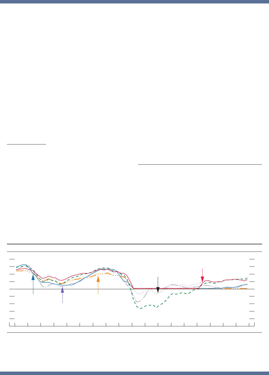
38 PART 2: MONETARY POLICY
Committee’s 2percent objective.
8
Rules that try to offset
the cumulative shortfall of accommodation posed by
the zero bound on interest rates, such as the adjusted
Taylor (1993) rule, or make up the cumulative shortfall
in the level of prices, such as the price-level rule, are
intended to help achieve average ination at or near
2percent over time.
9
Different monetary policy rules often offer quite
different prescriptions for the federal funds rate, and
there is no unambiguous metric for favoring one rule
over another. While monetary policy rules often agree
about the direction (up or down) in which policymakers
should move the federal funds rate, they frequently
disagree about the appropriate level of that rate.
Historical prescriptions from policy rules differ from
one another and also differ from the Committee’s target
for the federal funds rate, as shown in gure C. (These
prescriptions are calculated using both the actual data
and the estimates of the neutral real interest rate in
the longer run and of the rate of unemployment in the
longer run—data and estimates that were available to
FOMC policymakers at the time.) Moreover, the rules
sometimes prescribe setting short-term interest rates
well below zero—a setting that is not feasible. With
the exception of the adjusted Taylor (1993) and price-
level rules, which impose a lower limit of zero, all of
the rules shown in gureC called for the federal funds
rate to turn negative in 2009 and to stay below zero
for several years thereafter. Thus, these rules indicated
that the Federal Reserve should provide more monetary
stimulus than could be achieved by setting the federal
funds rate at zero. Almost all of the policy rules have
called for rising values of the federal funds rate in
recent years, but the pace of tightening that the rules
prescribe has varied widely. Prescriptions from these
rules for the level of the federal funds rate in the fourth
quarter of 2017 ranged from 0 basis points (price-level
rule) to 3.0percent (balanced-approach rule).
10
First-difference rule
Price-level ruleTarget federal funds rate
Balanced-approach rule
Taylor (1993) rule, adjusted
8
6
4
2
+
_
0
2
4
6
8
Percent
201720152013201120092007200520032001
C. Historical federal funds rate prescriptions from simple policy rules
Quarterly
Taylor (1993) rule
N
OTE: The rules use real-time historical values of inflation, the federal funds rate, and the unemployment rate. Inflation is measur
ed as the four-quarter percent
change
in the price index for personal consumption expenditures excluding food and energy. Quarterly projections of long-run values for the federal funds
rate
and
the unemployment rate are derived through interpolations of biannual projections from Blue Chip Economic Indicators. The long-run value for inflation
is
taken
as 2 percent. The target value of the price level is the average level of the price index for personal consumption expenditures excluding food and energy
in
1998, extrapolated at 2 percent per year.
SOURCE
: Federal Reserve Bank of Philadelphia; Wolters Kluwer, Blue Chip Economic Indicators; Federal Reserve Board staff estimates.
8. For further discussion of these issues, see Michael T.
Kiley and John M. Roberts (2017), “Monetary Policy in a Low
Interest Rate World,” Brookings Papers on Economic Activity,
Spring, pp. 317–72, https://www.brookings.edu/wp-content/
uploads/2017/08/kileytextsp17bpea.pdf.
9. Economists have found that a “makeup” policy can
be the best response in theory when the policy interest
rate is constrained at zero. See Ben S. Bernanke (2017),
“Monetary Policy in a New Era,” paper presented at
“Rethinking Macroeconomic Policy,” a conference held at the
Peterson Institute for International Economics, Washington,
October12–13, https://www.brookings.edu/wp-content/
uploads/2017/10/bernanke_rethinking_macro_nal.pdf;
and Michael Woodford (1999), “Commentary: How Should
Monetary Policy Be Conducted in an Era of Price Stability?”
Monetary Policy Rules and Their Role (continued)
in New Challenges for Monetary Policy, proceedings of a
symposium sponsored by the Federal Reserve Bank of Kansas
City, held in Jackson Hole, Wyo., August26–28 (Kansas
City: Federal Reserve Bank of Kansas City), pp.277–316,
https://www.kansascityfed.org/publications/research/escp/
symposiums/escp-1999.
10. As noted earlier, the price-level rule makes up for the
cumulative shortfall in the price level when ination runs
below 2percent. Because ination has been below 2percent
in recent years, the price-level rule calls for the federal funds
rate to remain at zero.

39
Part 3
summary of economic Projections
The following material appeared as an addendum to the minutes of the December12–13, 2017,
meeting of the Federal Open Market Committee.
In conjunction with the Federal Open
Market Committee (FOMC) meeting held on
December12–13, 2017, meeting participants
submitted their projections of the most likely
outcomes for real gross domestic product
(GDP) growth, the unemployment rate, and
ination for each year from 2017 to 2020
and over the longer run.
13
Each participant’s
projection was based on information available
at the time of the meeting, together with his
or her assessment of appropriate monetary
policy—including a path for the federal
funds rate and its longer-run value—and
assumptions about other factors likely to
aect economic outcomes. The longer-run
projections represent each participant’s
assessment of the value to which each variable
would be expected to converge, over time,
under appropriate monetary policy and in the
absence of further shocks to the economy.
14
“Appropriate monetary policy” is dened as
the future path of policy that each participant
deems most likely to foster outcomes for
economic activity and ination that best
satisfy his or her individual interpretation of
the statutory mandate to promote maximum
employment and price stability.
All participants who submitted longer-run
projections expected that, under appropriate
13. Four members of the Board of Governors were
in oce at the time of the December2017 meeting, the
same number as in September2017. However, since
the September meeting, one member, Stanley Fischer,
resigned from the Board and another, Randal K. Quarles,
joined. The incoming president of the Federal Reserve
Bank of Richmond is scheduled to assume oce on
January1, 2018; First Vice President Mark L. Mullinix
submitted economic projections at this meeting as he did
in September.
14. One participant did not submit longer-run
projections for real output growth, the unemployment
rate, or the federal funds rate.
monetary policy, growth in real GDP in
2018 would be somewhat stronger than their
individual estimates of its longer-run rate.
All participants projected that real GDP
growth would moderate in 2019, and nearly
all predicted that it would ease further in
2020; a solid majority of participants thought
that growth in real GDP would be at or
close to their individual estimates of the
economy’s longer-run growth rate by 2020.
All participants who submitted longer-run
projections expected that the unemployment
rate would run below their estimates of
its longer-run normal level through 2020.
Participants generally projected that ination,
as measured by the four-quarter percentage
change in the price index for personal
consumption expenditures (PCE), would
step up toward the Committee’s 2percent
objective in 2018 and be at or close to that
objective by 2019. Most participants indicated
that prospective changes in federal tax policy
were a factor that led them to boost their
projections of real GDP growth over the next
couple of years; some participants, however,
noted that they had already incorporated at
least some eects of future tax cuts in their
September projections. Several also noted the
possibility that changes to tax policy could
raise the level of potential GDP in the longer
run.
15
Table1 and gure1 provide summary
statistics for the projections.
As shown in gure2, participants generally
expected that the evolution of the economy
relative to their objectives of maximum
employment and 2percent ination would
15. Participants completed their submissions for
the Summary of Economic Projections before the
reconciliation of the House and Senate tax bills in the
Congress.

40 PART 3: SUMMARY OF ECONOMIC PROJECTIONS
likely warrant further gradual increases in
the federal funds rate. Compared with the
projections they submitted in September,
some participants raised their federal funds
rate projections for 2018 and 2019, while
several others lowered their projections, leaving
the median projection for the federal funds
rate in those years unchanged; the median
projection for 2020 was slightly higher, and the
median projection for the longer-run normal
level of the federal funds rate was unchanged.
Nearly all participants saw it as likely to be
appropriate for the federal funds rate to rise
above their estimates of its longer-run normal
level at some point during the forecast period.
Participants generally noted several sources
of uncertainty about the future course of
the federal funds rate, including the details
of potential changes in tax policy, how those
changes would aect the economy, and the
range of factors inuencing ination over the
medium term.
In general, participants viewed the uncertainty
attached to their economic projections
as broadly similar to the average of the
past 20years, and all participants saw the
uncertainty associated with their projections
for real GDP growth, the unemployment rate,
and ination as essentially unchanged from
September. As in September, most participants
judged the risks around their projections for
economic growth, the unemployment rate, and
ination as broadly balanced.
The Outlook for Economic Activity
The median of participants’ projections for the
growth rate of real GDP for 2018, conditional
on their individual assessments of appropriate
monetary policy, was 2.5percent, the same
as for 2017. The median projections for GDP
growth in 2019 and 2020 were slightly lower,
at 2.1 and 2.0percent, respectively. Compared
with the Summary of Economic Projections
(SEP) from September, the median of the
projections for real GDP growth for 2018
was notably higher, while the medians for real
GDP growth for 2019 and 2020 were modestly
higher. The median of projections for the
Table 1. Economic projections of Federal Reserve Board members and Federal Reserve Bank presidents, under their
individual assessments of projected appropriate monetary policy, December2017
Percent
Variable
Median
1
Central tendency
2
Range
3
2017 2018 2019 2020
Longer
run
2017 2018 2019 2020
Longer
run
2017 2018 2019 2020
Longer
run
Change in real GDP ..... 2.5 2.5 2.1 2.0 1.8 2.4–2.5 2.2–2.6 1.9–2.3 1.7–2.0 1.8–1.9 2.4–2.6 2.2–2.8 1.7–2.4 1.1–2.2 1.7–2.2
September projection .. 2.4 2.1 2.0 1.8 1.8 2.2–2.5 2.0–2.3 1.7–2.1 1.6–2.0 1.8–2.0 2.2–2.7 1.7–2.6 1.4 –2.3 1.4 –2.0 1.5–2.2
Unemployment rate. . . . . . 4.1 3.9 3.9 4.0 4.6 4.1 3.7–4.0 3.6–4.0 3.6–4.2 4.4–4.7 4.1 3.6–4.0 3.5–4.2 3.5–4.5 4.3–5.0
September projection .. 4.3 4.1 4.1 4.2 4.6 4.2–4.3 4.0–4.2 3.9–4.4 4.0–4.5 4.5–4.8 4.2–4.5 3.9–4.5 3.8–4.5 3.8–4.8 4.4–5.0
PCE ination ............ 1.7 1.9 2.0 2.0 2.0 1.6 –1.7 1.7–1.9 2.0 2.0–2.1 2.0 1.5–1.7 1.7–2.1 1.8–2.3 1.9–2.2 2.0
September projection .. 1.6 1.9 2.0 2.0 2.0 1.5–1.6 1.8–2.0 2.0 2.0–2.1 2.0 1.5–1.7 1.7–2.0 1.8–2.2 1.9–2.2 2.0
Core PCE ination
4
...... 1.5 1.9 2.0 2.0 1.5 1.7–1.9 2.0 2.0–2.1 1.4 –1.5 1.7–2.0 1.8–2.3 1.9–2.3
September projection .. 1.5 1.9 2.0 2.0 1.5–1.6 1.8–2.0 2.0 2.0–2.1 1.4–1.7 1.7–2.0 1.8–2.2 1.9–2.2
Memo: Projected
appropriate policy path
Federal funds rate ....... 1.4 2.1 2.7 3.1 2.8 1.4 1.9–2.4 2.4–3.1 2.6 –3.1 2.8–3.0 1.1–1.4 1.1–2.6 1.4 –3.6 1.4–4.1 2.3–3.0
September projection .. 1.4 2.1 2.7 2.9 2.8 1.1–1.4 1.9–2.4 2.4–3.1 2.5–3.5 2.5–3.0 1.1–1.6 1.1–2.6 1.1–3.4 1.1–3.9 2.3–3.5
N: Projections of change in real gross domestic product (GDP) and projections for both measures of ination are percent changes from the fourth quarter of the previous year to
the fourth quarter of the year indicated. PCE ination and core PCE ination are the percentage rates of change in, respectively, the price index for personal consumption expenditures
(PCE) and the price index for PCE excluding food and energy. Projections for the unemployment rate are for the average civilian unemployment rate in the fourth quarter of the year
indicated. Each participant’s projections are based on his or her assessment of appropriate monetary policy. Longer-run projections represent each participant’s assessment of the rate
to which each variable would be expected to converge under appropriate monetary policy and in the absence of further shocks to the economy. The projections for the federal funds
rate are the value of the midpoint of the projected appropriate target range for the federal funds rate or the projected appropriate target level for the federal funds rate at the end of the
specied calendar year or over the longer run. The September projections were made in conjunction with the meeting of the Federal Open Market Committee on September19–20,
2017. One participant did not submit longer-run projections for the change in real GDP, the unemployment rate, or the federal funds rate in conjunction with the September19–20,
2017, meeting, and one participant did not submit such projections in conjunction with the December12–13, 2017, meeting.
1. For each period, the median is the middle projection when the projections are arranged from lowest to highest. When the number of projections is even, the median is the average
of the two middle projections.
2. The central tendency excludes the three highest and three lowest projections for each variable in each year.
3. The range for a variable in a given year includes all participants’ projections, from lowest to highest, for that variable in that year.
4. Longer-run projections for core PCE ination are not collected.
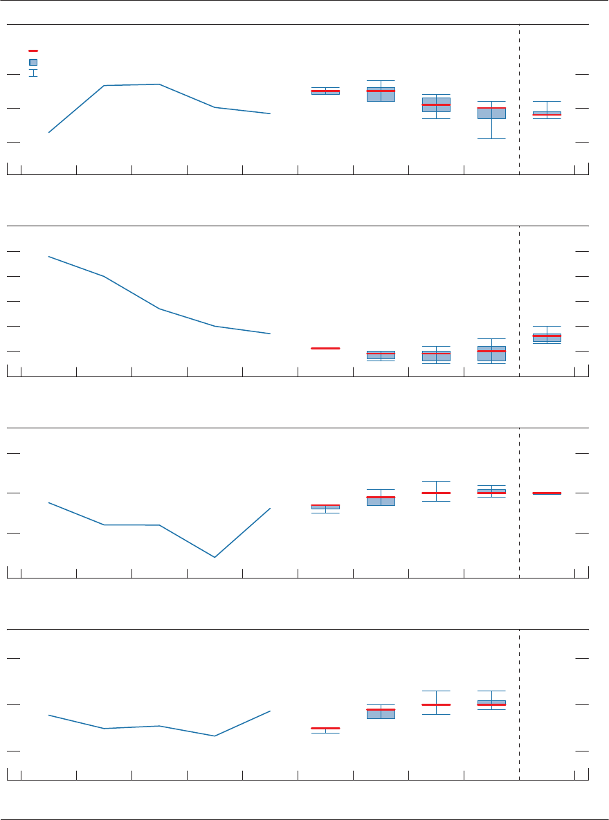
MONETARY POLICY REPORT: FEBRUARY 2018 41
Change in real GDP
Percent
1
2
3
2012 2013 2014 2015 2016 2017 2018 2019 2020
Longer
run
Median of projections
Central tendency of projections
Range of projections
Actual
Unemployment rate
Percent
4
5
6
7
8
2012 2013 2014 2015 2016 2017 2018 2019 2020
PCE ination
Percent
1
2
3
2012 2013 2014 2015 2016 2017 2018 2019 2020
Core PCE ination
Percent
1
2
3
2012 2013 2014 2015 2016 2017 2018 2019 2020
Figure 1. Medians, central tendencies, and ranges of economic projections, 2017–20 and over the longer run
N
: Denitions of variables and other explanations are in the notes to table 1. The data for the actual values of the variables
are annual.
Longer
run
Longer
run
Longer
run
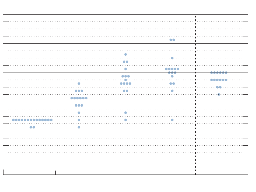
42 PART 3: SUMMARY OF ECONOMIC PROJECTIONS
longer-run normal rate of real GDP growth
remained at 1.8percent. Most participants
pointed to changes in tax policy as likely
to provide some boost to real GDP growth
over the forecast period; in September, fewer
than half of the participants incorporated
prospective tax policy changes in their
projections. Several participants indicated
that they had marked up their estimates of
the magnitude of tax cuts, relative to their
assumptions in September.
The medians of projections for the
unemployment rate in the fourth quarter
of both 2018 and 2019 were 3.9percent,
0.2percentage point below the medians from
September and about ¾percentage point
below the median assessment of its longer-
run normal level. The median projection for
the unemployment rate ticked up slightly to
4.0percent in 2020.
Figures 3.A and 3.B show the distributions of
participants’ projections for real GDP growth
and the unemployment rate from 2017 to 2020
and in the longer run. The distribution of
individual projections for real GDP growth
for 2018 shifted up, with more than half of
the participants now expecting real GDP
growth of 2.5percent or more and none
seeing it below 2.2percent. The distribution
of projected real GDP growth in 2019 and
2020 also shifted up, albeit only slightly. The
distribution for the longer-run normal rate
of GDP growth was little changed from
September. The distributions of individual
projections for the unemployment rate in
2018 and 2019 shifted down relative to those
Percent
0.0
0.5
1.0
1.5
2.0
2.5
3.0
3.5
4.0
4.5
5.0
2017 2018 2019 2020 Longer run
Figure 2. FOMC participants’ assessments of appropriate monetary policy: Midpoint of target range or target level
for the federal funds rate
N:
Each shaded circle indicates the value (rounded to the nearest 1/8 percentage point) of an individual participant’s
judgment of the midpoint of the appropriate target range for the federal funds rate or the appropriate target level for the federal
funds rate at the end of the specied calendar year or over the longer run. One participant did not submit longer-run projections
for the federal funds rate.
MONETARY POLICY REPORT: FEBRUARY 2018 43
2017
2
4
6
8
10
12
14
16
18
2018
2
4
6
8
10
12
14
16
18
2019
2
4
6
8
10
12
14
16
18
2020
2
4
6
8
10
12
14
16
18
Longer run
2
4
6
8
10
12
14
16
18
Percent range
Percent range
Percent range
Percent range
Percent range
Figure 3.A. Distribution of participants’ projections for the change in real GDP, 2017–20 and over the longer run
N: Denitions of variables and other explanations are in the notes to table 1.
Number of participants
Number of participants
Number of participants
Number of participants
Number of participants
1.0 – 1.2 – 1.4 – 1.6 – 1.8 – 2.0 – 2.2 – 2.4 – 2.6 – 2.8 –
1.1 1.3 1.5 1.7 1.9 2.1 2.3 2.5 2.7 2.9
1.0 – 1.2 – 1.4 – 1.6 – 1.8 – 2.0 – 2.2 – 2.4 – 2.6 – 2.8 –
1.1 1.3 1.5 1.7 1.9 2.1 2.3 2.5 2.7 2.9
1.0 – 1.2 – 1.4 – 1.6 – 1.8 – 2.0 – 2.2 – 2.4 – 2.6 – 2.8 –
1.1 1.3 1.5 1.7 1.9 2.1 2.3 2.5 2.7 2.9
1.0 – 1.2 – 1.4 – 1.6 – 1.8 – 2.0 – 2.2 – 2.4 – 2.6 – 2.8 –
1.1 1.3 1.5 1.7 1.9 2.1 2.3 2.5 2.7 2.9
1.0 – 1.2 – 1.4 – 1.6 – 1.8 – 2.0 – 2.2 – 2.4 – 2.6 – 2.8 –
1.1 1.3 1.5 1.7 1.9 2.1 2.3 2.5 2.7 2.9
December projections
September projections
44 PART 3: SUMMARY OF ECONOMIC PROJECTIONS
2
4
6
8
10
12
14
16
18
2
4
6
8
10
12
14
16
18
2
4
6
8
10
12
14
16
18
2
4
6
8
10
12
14
16
18
2
4
6
8
10
12
14
16
18
Figure 3.B. Distribution of participants’ projections for the unemployment rate, 2017–20 and over the longer run
N: Denitions of variables and other explanations are in the notes to table 1.
Number of participants
Number of participants
Number of participants
Number of participants
Number of participants
Percent range
Percent range
Percent range
Percent range
Percent range
2017
December projections
September projections
2018
2019
2020
Longer run
3.2 – 3.4 – 3.6 – 3.8 – 4.0 – 4.2 – 4.4 – 4.6 – 4.8 – 5.0 –
3.3 3.5 3.7 3.9 4.1 4.3 4.5 4.7 4.9 5.1
3.2 – 3.4 – 3.6 – 3.8 – 4.0 – 4.2 – 4.4 – 4.6 – 4.8 – 5.0 –
3.3 3.5 3.7 3.9 4.1 4.3 4.5 4.7 4.9 5.1
3.2 – 3.4 – 3.6 – 3.8 – 4.0 – 4.2 – 4.4 – 4.6 – 4.8 – 5.0 –
3.3 3.5 3.7 3.9 4.1 4.3 4.5 4.7 4.9 5.1
3.2 – 3.4 – 3.6 – 3.8 – 4.0 – 4.2 – 4.4 – 4.6 – 4.8 – 5.0 –
3.3 3.5 3.7 3.9 4.1 4.3 4.5 4.7 4.9 5.1
3.2 – 3.4 – 3.6 – 3.8 – 4.0 – 4.2 – 4.4 – 4.6 – 4.8 – 5.0 –
3.3 3.5 3.7 3.9 4.1 4.3 4.5 4.7 4.9 5.1
MONETARY POLICY REPORT: FEBRUARY 2018 45
in September, broadly consistent with the
changes in the distributions for real
GDP growth.
The Outlook for Ination
The median of projections for headline
PCE price ination was 1.9percent in 2018
and 2percent in 2019 and 2020, the same
as in the September SEP. Most participants
anticipated that ination would continue to
run a bit below 2percent in 2018, and only
one participant expected ination above
2percent that year. A majority of participants
projected that ination would be equal to
the Committee’s objective in 2019 and 2020.
Several participants projected that ination
would slightly exceed 2percent in 2019 or
2020. The medians of projections for core PCE
price ination over the 2018–20 period were
the same as those for headline ination.
Figures 3.C and 3.D provide information on
the distributions of participants’ views about
the outlook for ination. On the whole, the
distributions of projections for headline
PCE price ination and core PCE price
ination beyond 2017 were little changed
from September.
Appropriate Monetary Policy
Figure 3.E provides the distribution of
participants’ judgments regarding the
appropriate target—or midpoint of the target
range—for the federal funds rate at the end
of each year from 2017 to 2020 and in the
longer run. Overall, the distributions diered
in only small ways from those reported in
the September SEP. There was a moderate
reduction in the dispersion of the distribution
for 2020 and for the longer run; some of the
lower-end projections for those horizons from
the September SEP were revised up in the
current projections.
The median projection of the year-end federal
funds rate continued to rise gradually over the
2018–20 period. The median projection for the
end of 2018 was 2.13percent; the medians of
the projections were 2.69percent at the end
of 2019 and 3.07percent at the end of 2020.
Nearly all participants projected that it would
likely be appropriate for the federal funds
rate to rise above their individual estimates
of the longer-run normal rate at some point
over the forecast period. Compared with their
projections prepared for the September SEP,
a few participants raised their projections for
the federal funds rate in the longer run and
one lowered it; the median was unchanged at
2.75percent.
In discussing their projections, many
participants once again expressed the view
that the appropriate trajectory of the federal
funds rate over the next few years would
likely involve gradual increases. This view
was predicated on several factors, including a
judgment that the neutral real interest rate
was currently low and would move up only
slowly, as well as the balancing of risks
associated with, among other things, the
possibility that ination pressures could build
if the economy expands well beyond its long-
run sustainable level, and the possibility that
the forces depressing ination could prove to
be more persistent than currently anticipated.
As always, the actual path of the federal
funds rate will depend on evolving economic
conditions and their implications for the
economic outlook.
Uncertainty and Risks
In assessing the path for the federal funds rate
that, in their view, is likely to be appropriate,
FOMC participants take account of the
range of possible economic outcomes,
the likelihood of those outcomes, and the
potential benets and costs should they
occur. As a reference, table2 provides a
measure of forecast uncertainty, based on
the forecast errors of various private and
government forecasts over the past 20years,
for real GDP growth, the unemployment
rate, and total consumer price ination. That
measure is incorporated graphically in the
top panels of gures 4.A, 4.B, and 4.C, which
display “fan charts” plotting the median SEP
46 PART 3: SUMMARY OF ECONOMIC PROJECTIONS
2
4
6
8
10
12
14
16
18
2
4
6
8
10
12
14
16
18
2
4
6
8
10
12
14
16
18
2
4
6
8
10
12
14
16
18
2
4
6
8
10
12
14
16
18
Figure 3.C. Distribution of participants’ projections for PCE ination, 2017–20 and over the longer run
N: Denitions of variables and other explanations are in the notes to table 1.
Number of participants
Number of participants
Number of participants
Number of participants
Number of participants
Percent range
Percent range
Percent range
Percent range
Percent range
2017
December projections
September projections
2018
2019
2020
Longer run
1.5 – 1.7 – 1.9 – 2.1 – 2.3 –
1.6 1.8 2.0 2.2
2.4
1.5 – 1.7 – 1.9 – 2.1 – 2.3 –
1.6 1.8 2.0 2.2
2.4
1.5 – 1.7 – 1.9 – 2.1 – 2.3 –
1.6 1.8 2.0 2.2
2.4
1.5 – 1.7 – 1.9 – 2.1 – 2.3 –
1.6 1.8 2.0 2.2
2.4
1.5 – 1.7 – 1.9 – 2.1 – 2.3 –
1.6 1.8 2.0 2.2
2.4
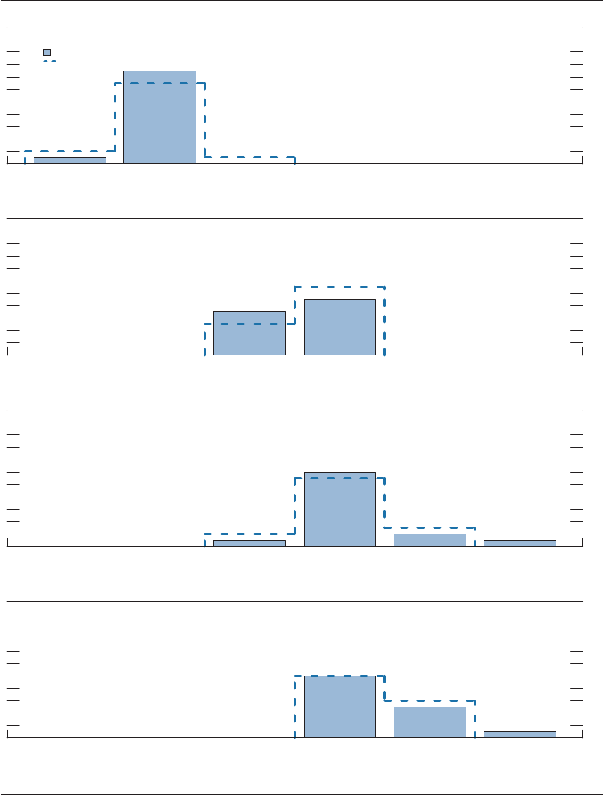
MONETARY POLICY REPORT: FEBRUARY 2018 47
2017
2
4
6
8
10
12
14
16
18
December projections
September projections
2018
2
4
6
8
10
12
14
16
18
2019
2
4
6
8
10
12
14
16
18
2020
2
4
6
8
10
12
14
16
18
Figure 3.D. Distribution of participants’ projections for core PCE ination, 2017–20
Percent range
Percent range
Percent range
Percent range
N: Denitions of variables and other explanations are in the notes to table 1.
Number of participants
Number of participants
Number of participants
Number of participants
1.3 – 1.5 – 1.7 – 1.9 – 2.1 – 2.3 –
1.4 1.6 1.8 2.0 2.2 2.4
1.3 – 1.5 – 1.7 – 1.9 – 2.1 – 2.3 –
1.4 1.6 1.8 2.0 2.2 2.4
1.3 – 1.5 – 1.7 – 1.9 – 2.1 – 2.3 –
1.4 1.6 1.8 2.0 2.2 2.4
1.3 – 1.5 – 1.7 – 1.9 – 2.1 – 2.3 –
1.4 1.6 1.8 2.0 2.2 2.4
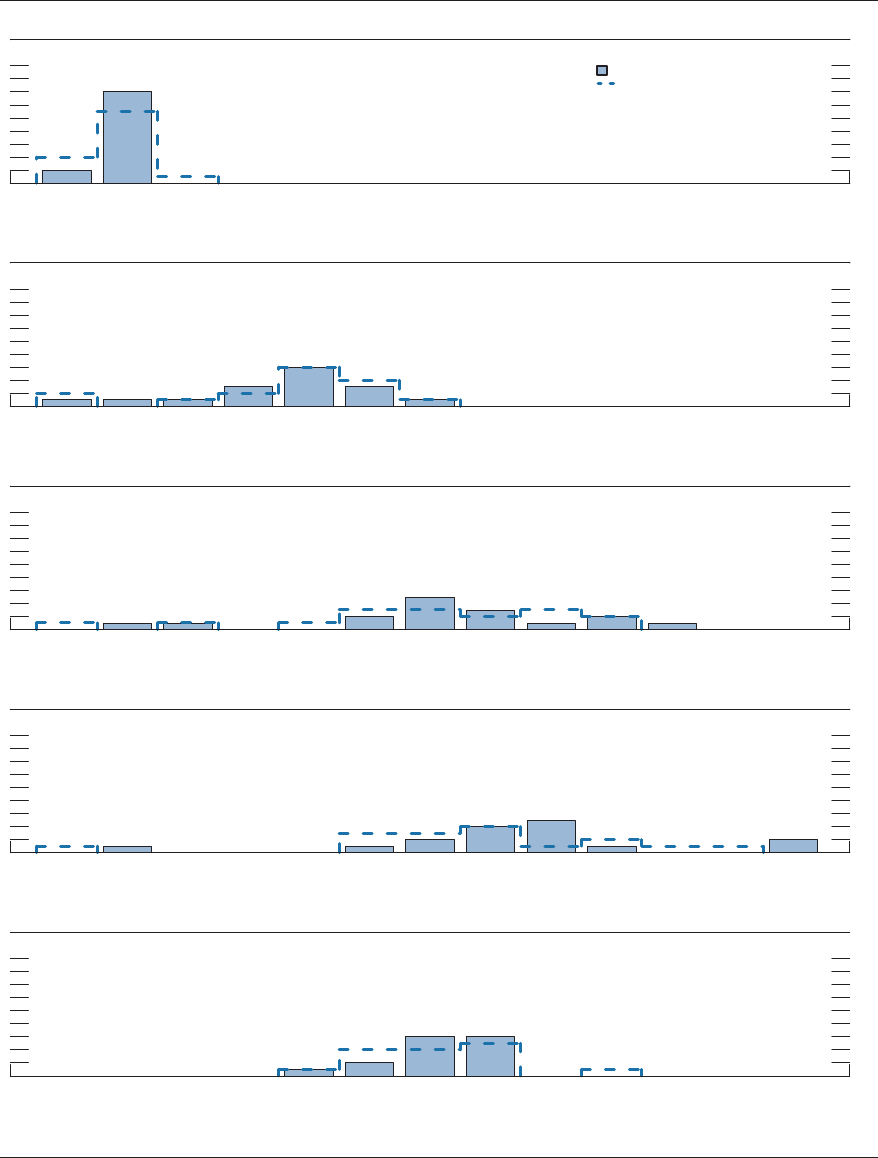
48 PART 3: SUMMARY OF ECONOMIC PROJECTIONS
2017
2
4
6
8
10
12
14
16
18
2018
2
4
6
8
10
12
14
16
18
2019
2
4
6
8
10
12
14
16
18
2020
2
4
6
8
10
12
14
16
18
Longer run
2
4
6
8
10
12
14
16
18
Number of participants
Number of participants
Number of participants
Number of participants
Number of participants
December projections
September projections
1.13 – 1.38 – 1.63 – 1.88 – 2.13 – 2.38 – 2.63 – 2.88 – 3.13 – 3.38 – 3.63 – 3.88 – 4.13 –
1.37 1.62 1.87 2.12 2.37 2.62 2.87 3.12 3.37 3.62 3.87 4.12 4.37
1.13 – 1.38 – 1.63 – 1.88 – 2.13 – 2.38 – 2.63 – 2.88 – 3.13 – 3.38 – 3.63 – 3.88 – 4.13 –
1.37 1.62 1.87 2.12 2.37 2.62 2.87 3.12 3.37 3.62 3.87 4.12 4.37
1.13 – 1.38 – 1.63 – 1.88 – 2.13 – 2.38 – 2.63 – 2.88 – 3.13 – 3.38 – 3.63 – 3.88 – 4.13 –
1.37 1.62 1.87 2.12 2.37 2.62 2.87 3.12 3.37 3.62 3.87 4.12 4.37
1.13 – 1.38 – 1.63 – 1.88 – 2.13 – 2.38 – 2.63 – 2.88 – 3.13 – 3.38 – 3.63 – 3.88 – 4.13 –
1.37 1.62 1.87 2.12 2.37 2.62 2.87 3.12 3.37 3.62 3.87 4.12 4.37
1.13 – 1.38 – 1.63 – 1.88 – 2.13 – 2.38 – 2.63 – 2.88 – 3.13 – 3.38 – 3.63 – 3.88 – 4.13 –
1.37 1.62 1.87 2.12 2.37 2.62 2.87 3.12 3.37 3.62 3.87 4.12 4.37
N: Denitions of variables and other explanations are in the notes to table 1.
Percent range
Percent range
Percent range
Percent range
Percent range
Figure 3.E. Distribution of participants’ judgments of the midpoint of the appropriate target range for the federal
funds rate or the appropriate target level for the federal funds rate, 2017–20 and over the longer run

MONETARY POLICY REPORT: FEBRUARY 2018 49
projections for the three variables surrounded
by symmetric condence intervals derived
from the forecast errors presented in table2.
If the degree of uncertainty attending these
projections is similar to the typical magnitude
of past forecast errors and the risks around
the projections are broadly balanced, future
outcomes of these variables would have
about a 70percent probability of occurring
within these condence intervals. For all
three variables, this measure of projection
uncertainty is substantial and generally
increases as the forecast horizon lengthens.
Participants’ assessments of the level of
uncertainty surrounding their economic
projections are shown in the bottom-left
panels of gures 4.A, 4.B, and 4.C. Nearly all
participants viewed the degree of uncertainty
attached to their economic projections about
GDP growth, the unemployment rate, and
ination as broadly similar to the average of
the past 20years, a view that was essentially
unchanged from September.
16
About half of
the participants who commented on this topic
suggested that uncertainties about the details
of the pending tax legislation had raised their
assessment of uncertainty for GDP growth,
albeit not by enough to tip their assessments
into the higher-than-average category.
Because the fan charts are constructed to be
symmetric around the median projection,
they do not reect any asymmetries in the
balance of risks that participants may see
in their economic projections. Accordingly,
participants’ assessments of the balance of
risks to their economic projections are shown
in the bottom-right panels of gures 4.A, 4.B,
and 4.C. As in September, most participants
judged the risks to their projections of
real GDP growth, the unemployment rate,
headline ination and core ination as
broadly balanced—in other words, as broadly
16. At the end of this summary, the box “Forecast
Uncertainty” discusses the sources and interpretation
of uncertainty in the economic forecasts and explains
the approach used to assess the uncertainty and risks
attending the participants’ projections.
consistent with a symmetric fan chart. The
balance of risks to the economic outlook
shifted slightly in the direction of strength,
with two more participants seeing upside risks
to growth in real GDP than in September and
one more seeing risks to the unemployment
rate as weighted to the downside. In addition,
one more participant than before saw risks to
ination as weighted to the upside.
Participants’ assessments of the future
path of the federal funds rate consistent
with appropriate policy are also subject
to considerable uncertainty. Because the
Committee adjusts the federal funds rate
in response to actual and prospective
developments over time in real GDP growth,
unemployment, and ination, uncertainty
surrounding the projected path for the funds
rate importantly reects the uncertainties
about the path for those key economic
variables. Figure5 provides a graphical
representation of this uncertainty, plotting
the median SEP projection for the federal
funds rate surrounded by condence intervals
derived from the results presented in table2.
As with the macroeconomic variables, forecast
uncertainty is substantial and increases for
longer horizons.
Table 2. Average historical projection error ranges
Percentage points
Variable 2017 2018 2019 2020
Change in real GDP
1
...... ±0.8 ±1.7 ±2.1 ±2.2
Unemployment rate
1
...... ±0.1 ±0.8 ±1.5 ±1.9
Total consumer prices
2
.... ±0.2 ±1.0 ±1.1 ±1.0
Short-term interest rates
3
. ±0.1 ±1.4 ±1.9 ±2.4
Note: Error ranges shown are measured as plus or minus the root mean squared
error of projections for 1997 through 2016 that were released in the winter by various
private and government forecasters. As described in the box “Forecast Uncertain-
ty,” under certain assumptions, there is about a 70percent probability that actual
outcomes for real GDP, unemployment, consumer prices, and the federal funds rate
will be in ranges implied by the average size of projection errors made in the past.
For more information, see David Reifschneider and Peter Tulip (2017), “Gauging
the Uncertainty of the Economic Outlook Using Historical Forecasting Errors: The
Federal Reserve’s Approach,” Finance and Economics Discussion Series 2017-020
(Washington: Board of Governors of the Federal Reserve System, February), www.
federalreserve.gov/econresdata/feds/2017/files/2017020pap.pdf.
1. Denitions of variables are in the general note to table1.
2. Measure is the overall consumer price index, the price measure that has been
most widely used in government and private economic forecasts. Projections are
percent changes on a fourth quarter to fourth quarter basis.
3. For Federal Reserve sta forecasts, measure is the federal funds rate. For other
forecasts, measure is the rate on 3-month Treasury bills. Projection errors are calculat-
ed using average levels, in percent, in the fourth quarter.
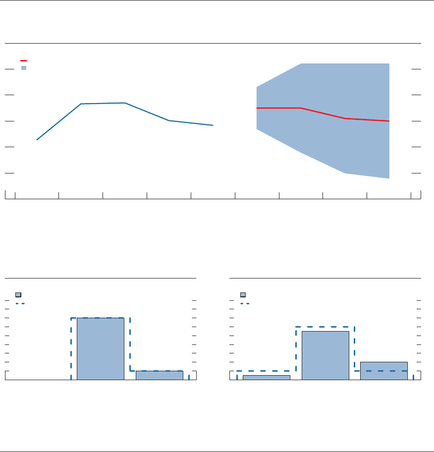
50 PART 3: SUMMARY OF ECONOMIC PROJECTIONS
Change in real GDP
Percent
0
1
2
3
4
2012 2013 2014 2015 2016 2017 2018 2019 2020
Actual
Uncertainty about GDP growth
2
4
6
8
10
12
14
16
18
Lower Broadly
similar
Higher
December projections
September projections
December projections
September projections
Risks to GDP growth
Number of participants
2
4
6
8
10
12
14
16
18
Weighted to
downside
Broadly
balanced
N: The blue and red lines in the top panel show actual values and median projected values, respectively, of the percent
change in real gross domestic product (GDP) from the fourth quarter of the previous year to the fourth quarter of the year
indicated. The condence interval around the median projected values is assumed to be symmetric and is based on root mean
squared errors of various private and government forecasts made over the previous 20 years; more information about these data
is available in table 2. Because current conditions may dier from those that prevailed, on average, over the previous 20 years,
the width and shape of the condence interval estimated on the basis of the historical forecast errors may not reect FOMC
participants’ current assessments of the uncertainty and risks around their projections; these current assessments are summarized
in the lower panels. Generally speaking, participants who judge the uncertainty about their projections as “broadly similar” to
the average levels of the past 20 years would view the width of the condence interval shown in the historical fan chart as largely
consistent with their assessments of the uncertainty about their projections. Likewise, participants who judge the risks to their
projections as “broadly balanced” would view the condence interval around their projections as approximately symmetric. For
denitions of uncertainty and risks in economic projections, see the box “Forecast Uncertainty.”
Figure 4.A. Uncertainty and risks in projections of GDP growth
Median projection and condence interval based on historical forecast errors
FOMC participants’ assessments of uncertainty and risks around their economic projections
Median of projections
70% condence interval
Number of participants
Weighted to
upside
MONETARY POLICY REPORT: FEBRUARY 2018 51
Figure 4.B. Uncertainty and risks in projections of the unemployment rate
Median projection and condence interval based on historical forecast errors
Unemployment rate
Percent
1
2
3
4
5
6
7
8
9
10
2012 2013 2014 2015 2016 2017 2018 2019 2020
Actual
FOMC participants’ assessments of uncertainty and risks around their economic projections
Uncertainty about the unemployment rate
Number of participants Number of participants
2
4
6
8
10
12
14
16
18
Risks to the unemployment rate
2
4
6
8
10
12
14
16
18
Median of projections
70% condence interval
December projections
September projections
December projections
September projections
Weighted to
downside
Broadly
balanced
Weighted to
upside
Lower Broadly
similar
Higher
N: The blue and red lines in the top panel show actual values and median projected values, respectively, of the average
civilian unemployment rate in the fourth quarter of the year indicated. The condence interval around the median projected
values is assumed to be symmetric and is based on root mean squared errors of various private and government forecasts made
over the previous 20 years; more information about these data is available in table 2. Because current conditions may dier
from those that prevailed, on average, over the previous 20 years, the width and shape of the condence interval estimated on
the basis of the historical forecast errors may not reect FOMC participants’ current assessments of the uncertainty and risks
around their projections; these current assessments are summarized in the lower panels. Generally speaking, participants who
judge the uncertainty about their projections as “broadly similar” to the average levels of the past 20 years would view the
width of the condence interval shown in the historical fan chart as largely consistent with their assessments of the uncertainty
about their projections. Likewise, participants who judge the risks to their projections as “broadly balanced” would view the
condence interval around their projections as approximately symmetric. For denitions of uncertainty and risks in economic
projections, see the box “Forecast Uncertainty.”
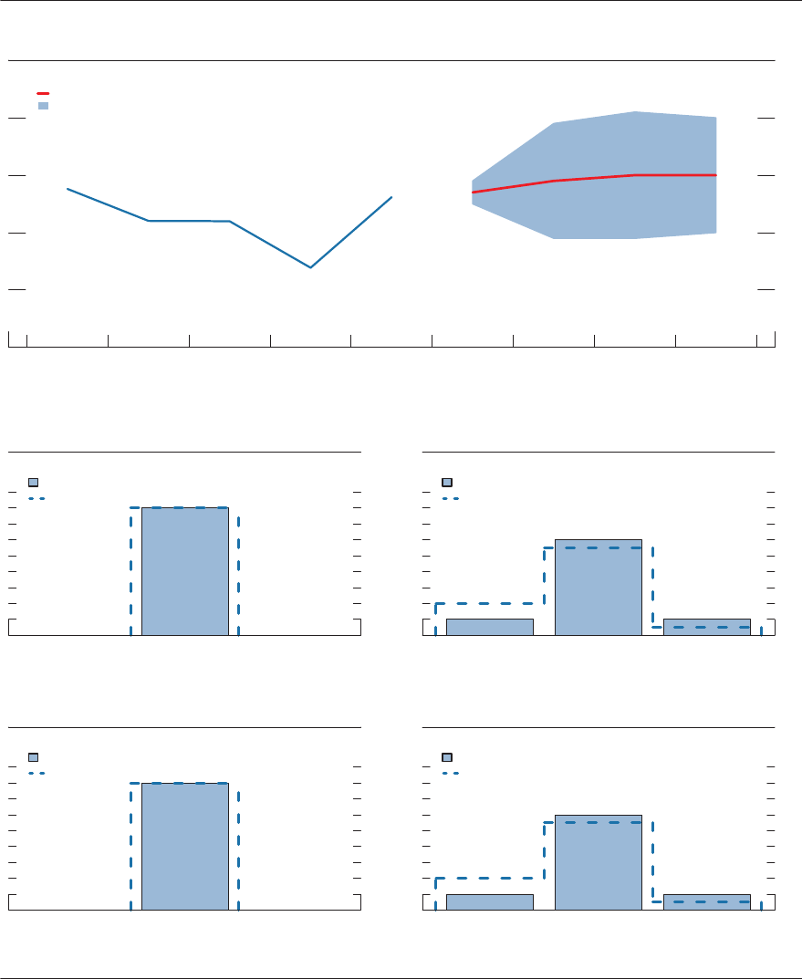
52 PART 3: SUMMARY OF ECONOMIC PROJECTIONS
PCE ination
Percent
0
1
2
3
2012 2013 2014 2015 2016 2017 2018 2019 2020
Actual
FOMC participants’ assessments of uncertainty and risks around their economic projections
Uncertainty about PCE ination
2
4
6
8
10
12
14
16
18
Uncertainty about core PCE ination
2
4
6
8
10
12
14
16
18
Risks to PCE ination
2
4
6
8
10
12
14
16
18
Risks to core PCE ination
2
4
6
8
10
12
14
16
18
Figure 4.C. Uncertainty and risks in projections of PCE ination
Median projection and condence interval based on historical forecast errors
Median of projections
70% condence interval
Weighted to
downside
Broadly
balanced
Weighted to
upside
Lower Broadly
similar
Higher
Weighted to
downside
Broadly
balanced
Weighted to
upside
Lower Broadly
similar
Higher
Number of participants Number of participants
Number of participants Number of participants
December projections
September projections
December projections
September projections
December projections
September projections
December projections
September projections
N: The blue and red lines in the top panel show actual values and median projected values, respectively, of the percent
change in the price index for personal consumption expenditures (PCE) from the fourth quarter of the previous year to the fourth
quarter of the year indicated. The condence interval around the median projected values is assumed to be symmetric and is based
on root mean squared errors of various private and government forecasts made over the previous 20 years; more information
about these data is available in table 2. Because current conditions may dier from those that prevailed, on average, over the
previous 20 years, the width and shape of the condence interval estimated on the basis of the historical forecast errors may not
reect FOMC participants’ current assessments of the uncertainty and risks around their projections; these current assessments
are
summarized in the lower panels. Generally speaking, participants who judge the uncertainty about their projections as “broadly
similar” to the average levels of the past 20 years would view the width of the condence interval shown in the historical fan chart
as largely consistent with their assessments of the uncertainty about their projections. Likewise, participants who judge the risks to
their projections as “broadly balanced” would view the condence interval around their projections as approximately symmetric.
For denitions of uncertainty and risks in economic projections, see the box “Forecast Uncertainty.”
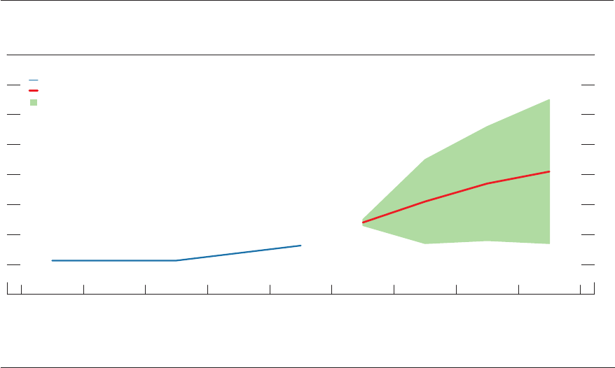
MONETARY POLICY REPORT: FEBRUARY 2018 53
Federal funds rate
Percent
0
1
2
3
4
5
6
2012 2013 2014 2015 2016 2017 2018 2019 2020
Midpoint of target range
Median of projections
70% condence interval*
Actual
Figure 5. Uncertainty in projections of the federal funds rate
Median projection and condence interval based on historical forecast errors
N
: The blue and red lines are based on actual values and median projected values, respectively, of the Committee’s target for
the federal funds rate at the end of the year indicated. The actual values are the midpoint of the target range; the median projected
values are based on either the midpoint of the target range or the target level. The condence interval around the median projected
values is based on root mean squared errors of various private and government forecasts made over the previous 20 years. The
condence interval is not strictly consistent with the projections for the federal funds rate, primarily because these projections are
not forecasts of the likeliest outcomes for the federal funds rate, but rather projections of participants’ individual assessments of
appropriate monetary policy. Still, historical forecast errors provide a broad sense of the uncertainty around the future path of the
federal funds rate generated by the uncertainty about the macroeconomic variables as well as additional adjustments to monetary
policy that may be appropriate to oset the eects of shocks to the economy.
The condence interval is assumed to be symmetric except when it is truncated at zero—the bottom of the lowest target range
for the federal funds rate that has been adopted in the past by the Committee. This truncation would not be intended to indicate
the likelihood of the use of negative interest rates to provide additional monetary policy accommodation if doing so was judged
appropriate. In such situations, the Committee could also employ other tools, including forward guidance and large-scale asset
purchases, to provide additional accommodation. Because current conditions may dier from those that prevailed, on average,
over the previous 20 years, the width and shape of the condence interval estimated on the basis of the historical forecast errors
may not reect FOMC participants’ current assessments of the uncertainty and risks around their projections.
* The condence interval is derived from forecasts of the average level of short-term interest rates in the fourth quarter of the
year indicated; more information about these data is available in table 2. The shaded area encompasses less than a 70 percent
condence interval if the condence interval has been truncated at zero.

54 PART 3: SUMMARY OF ECONOMIC PROJECTIONS
uncertainty surrounding their projections are summarized
in the bottom-left panels of those gures. Participants
also provide judgments as to whether the risks to their
projections are weighted to the upside, are weighted to
the downside, or are broadly balanced. That is, while the
symmetric historical fan charts shown in the top panels of
gures4.A through 4.C imply that the risks to participants’
projections are balanced, participants may judge that
there is a greater risk that a given variable will be above
rather than below their projections. These judgments
are summarized in the lower-right panels of gures 4.A
through 4.C.
As with real activity and ination, the outlook for
the future path of the federal funds rate is subject to
considerable uncertainty. This uncertainty arises primarily
because each participant’s assessment of the appropriate
stance of monetary policy depends importantly on
the evolution of real activity and ination over time. If
economic conditions evolve in an unexpected manner,
then assessments of the appropriate setting of the federal
funds rate would change from that point forward. The
nal line in table2 shows the error ranges for forecasts of
short-term interest rates. They suggest that the historical
condence intervals associated with projections of the
federal funds rate are quite wide. It should be noted,
however, that these condence intervals are not strictly
consistent with the projections for the federal funds
rate, as these projections are not forecasts of the most
likely quarterly outcomes but rather are projections
of participants’ individual assessments of appropriate
monetary policy and are on an end-of-year basis.
However, the forecast errors should provide a sense of the
uncertainty around the future path of the federal funds rate
generated by the uncertainty about the macroeconomic
variables as well as additional adjustments to monetary
policy that would be appropriate to offset the effects of
shocks to the economy.
If at some point in the future the condence interval
around the federal funds rate were to extend below zero,
it would be truncated at zero for purposes of the fan chart
shown in gure5; zero is the bottom of the lowest target
range for the federal funds rate that has been adopted
by the Committee in the past. This approach to the
construction of the federal funds rate fan chart would be
merely a convention; it would not have any implications
for possible future policy decisions regarding the use of
negative interest rates to provide additional monetary
policy accommodation if doing so were appropriate. In
such situations, the Committee could also employ other
tools, including forward guidance and asset purchases, to
provide additional accommodation.
While gures 4.A through 4.C provide information on
the uncertainty around the economic projections, gure1
provides information on the range of views across FOMC
participants. A comparison of gure1 with gures4.A
through 4.C shows that the dispersion of the projections
across participants is much smaller than the average
forecast errors over the past 20years.
The economic projections provided by the members of
the Board of Governors and the presidents of the Federal
Reserve Banks inform discussions of monetary policy
among policymakers and can aid public understanding
of the basis for policy actions. Considerable uncertainty
attends these projections, however. The economic and
statistical models and relationships used to help produce
economic forecasts are necessarily imperfect descriptions
of the real world, and the future path of the economy
can be affected by myriad unforeseen developments and
events. Thus, in setting the stance of monetary policy,
participants consider not only what appears to be the
most likely economic outcome as embodied in their
projections, but also the range of alternative possibilities,
the likelihood of their occurring, and the potential costs to
the economy should they occur.
Table 2 summarizes the average historical accuracy
of a range of forecasts, including those reported in past
Monetary Policy Reports and those prepared by the
Federal Reserve Board’s staff in advance of meetings
of the Federal Open Market Committee (FOMC). The
projection error ranges shown in the table illustrate the
considerable uncertainty associated with economic
forecasts. For example, suppose a participant projects that
real gross domestic product (GDP) and total consumer
prices will rise steadily at annual rates of, respectively,
3percent and 2percent. If the uncertainty attending those
projections is similar to that experienced in the past and
the risks around the projections are broadly balanced, the
numbers reported in table2 would imply a probability of
about 70percent that actual GDP would expand within
a range of 2.2 to 3.8percent in the current year, 1.3 to
4.7percent in the second year, 0.9 to 5.1percent in the
third year, and 0.8 to 5.2percent in the fourth year. The
corresponding 70percent condence intervals for overall
ination would be 1.8 to 2.2percent in the current year,
1.0 to 3.0percent in the second year, 0.9 to 3.1percent
in the third year, and 1.0 to 3.0percent in the fourth
year. Figures 4.A through 4.C illustrate these condence
bounds in “fan charts” that are symmetric and centered on
the medians of FOMC participants’ projections for GDP
growth, the unemployment rate, and ination. However,
in some instances, the risks around the projections may
not be symmetric. In particular, the unemployment rate
cannot be negative; furthermore, the risks around a
particular projection might be tilted to either the upside or
the downside, in which case the corresponding fan chart
would be asymmetrically positioned around the median
projection.
Because current conditions may differ from those that
prevailed, on average, over history, participants provide
judgments as to whether the uncertainty attached to
their projections of each economic variable is greater
than, smaller than, or broadly similar to typical levels
of forecast uncertainty seen in the past 20years, as
presented in table2 and reected in the widths of the
condence intervals shown in the top panels of gures4.A
through 4.C. Participants’ current assessments of the
Forecast Uncertainty
55
AFE advanced foreign economy
BOE Bank of England
C&I commercial and industrial
EME emerging market economy
FOMC Federal Open Market Committee; also, the Committee
GDP gross domestic product
LFPR labor force participation rate
MBS mortgage-backed securities
Michigan survey University of Michigan Surveys of Consumers
ON RRP overnight reverse repurchase agreement
OPEC Organization of the Petroleum Exporting Countries
PCE personal consumption expenditures
SEP Summary of Economic Projections
SLOOS Senior Loan Ocer Opinion Survey on Bank Lending Practices
SOMA System Open Market Account
S&P Standard & Poor’s
TCJA Tax Cuts and Jobs Act
TIPS Treasury Ination-Protected Securities
abbreviations

Board of Governors of the Federal Reserve System
For use at 11:00 a.m., EST
February 23, 2018
Monetary Policy rePort
February 23, 2018
